# Patterns and structures
This page gives the fields of `PatternData`, which holds a measured pattern, of `Structure` and the phases, cells and atoms inside it, and of `Parameter`, which holds every number a fit can refine.
[The instrument](instrument.html.md) gives the third object a refinement needs.
The [parameter map](parameters.html.md) gives the name a plan uses for each refinable number, with its unit and typical range.
Every object on this page refuses a field it does not know, so a misspelled keyword raises when the object is built.
Bounds are checked when the object is built, too, and not when the fit starts.
## Parameter
| Field | Type | Default | Meaning |
|---|---|---|---|
| `Parameter.value` | `float` | required | the current value, in `Parameter.unit` |
| `Parameter.vary` | `bool` | `False` | whether the fit refines it |
| `Parameter.min` | `float` | `-inf` | inclusive lower bound |
| `Parameter.max` | `float` | `inf` | inclusive upper bound |
| `Parameter.unit` | `str` or `None` | `None` | a label; nothing converts by it |
| `Parameter.stderr` | `float` or `None` | `None` | the esd, written by the fit |
| `Parameter.expr` | `str` or `None` | `None` | reserved for constraint expressions; anything but `None` raises |
`value` must lie within the bounds, and `min` must not exceed `max`.
An infinite bound survives a JSON round trip as `"Infinity"`, so an unbounded parameter can be saved.
```python
from rietx import Parameter
a = Parameter(value=4.15689, min=4.0, max=4.3, vary=True, unit="A")
width = Parameter.positive(1e-3, vary=True, unit="deg^2")
assert width.min == 0.0
```
`Parameter.positive` builds a quantity with no meaning below zero, such as a peak width, a scale or an absorption coefficient.
It sets `min=0.0`.
Each field that holds a `Parameter` declares its own range and unit.
A `Parameter` you pass to that field inherits the `min`, `max` and `unit` you left out, and a bound you state yourself wins.
So `occ=Parameter(value=1.0, vary=True)` on an `Atom` keeps the occupancy’s floor of 0 and no upper bound.
Each parameter refines in its own unit, and the fit holds `min` and `max` as a box.
A value the data push past a bound ends exactly on it.
> **Warning**
>
> A `min=0.0` parameter can end at exactly `0.0`.
> That is harmless where zero is the off state, as for a width or an extinction coefficient.
> Where the physics divides by the value, the parameter carries a floor above zero instead.
> `PreferredOrientation.r` stops at `MARCH_R_MIN` (1e-6), a hump’s width at `HUMP_FWHM_MIN` (0.1°), and `ProfileTCHZ.w` at 1e-8 deg².
`stderr` is the only field a fit writes back.
It is `None` on a parameter that was never free, and on a free one whose esd could not be estimated.
[About correlations and esds](../concepts/correlations.html.md) says when an esd is absent.
## Pattern
`PatternData` is the measurement: an abscissa, the intensity at each point, and what is known about its uncertainty.
| Field | Type | Default | Meaning |
|---|---|---|---|
| `PatternData.two_theta` | `list[float]` or `None` | `None` | 2θ in degrees, strictly increasing |
| `PatternData.tof` | `list[float]` or `None` | `None` | neutron flight time in µs, strictly increasing |
| `PatternData.intensity` | `list[float]` | required | measured intensity, one value per point |
| `PatternData.sigma` | `list[float]` or `None` | `None` | per-point esd from the file; `None` selects the Poisson fallback |
| `PatternData.excluded_regions` | `list[tuple[float, float]]` | `[]` | intervals left out of the fit, on whichever axis is set |
| `PatternData.metadata` | `dict[str, str]` | `{}` | what the reader found in the file header |
Exactly one of `two_theta` and `tof` is set, and a pattern that sets both or neither is refused.
A pattern needs at least two points, and `sigma` needs one value per point.
An excluded region whose ends are reversed or equal is refused.
`PatternData.axis` says which abscissa a pattern carries, `"two_theta"` or `"tof"`.
It is read from the field the reader filled in and never from the values.
A flight-time range of 1000-10000 µs passes every check that a 10-100° scan passes.
`PatternData.axis_unit` names the unit, for a message or an axis label.
The abscissa must increase strictly, and nothing sorts it for you.
A reader reverses a file stored high to low, and reports that it did.
A 2θ column that is not monotonic is refused, because sorting it, concatenating it and splitting it are three different measurements.
### Arrays
Six methods return numpy arrays.
| Method | Returns |
|---|---|
| `PatternData.x` | whichever abscissa is set, for code that windows, masks or counts channels |
| `PatternData.tt` | 2θ in degrees; raises on a time-of-flight pattern |
| `PatternData.tof_us` | flight time in µs; raises on a 2θ pattern |
| `PatternData.y` | the intensity |
| `PatternData.sig` | the σ that every weighted quantity divides by |
| `PatternData.in_range_mask` | `True` at each point the excluded regions leave in the fit |
```python
from rietx import PatternData
data = PatternData(two_theta=[10.0, 10.02, 10.04], intensity=[120.0, 480.0, 0.0])
print(data.sig().round(4))
print(data)
```
```text
[10.9545 21.9089 1. ]
PatternData of 3 points, 10–10.04° 2θ, median step 0.02°
intensity: [120, 480, 0]
sigma: None
excluded_regions: none
metadata: none
```
`sig()` returns the file’s `sigma` where the file had one, and √max(y, 1) where it did not.
The objective [(8.1)](../theory/estimation.html.md#equation-est-obj), every difference curve and both GUI windows divide by it.
The Poisson fallback is right for raw counts, and wrong by √t for intensities already divided by a counting time t.
A reader that cannot establish the intensity scale withholds σ and says so with [`PATTERN_INTENSITY_SCALED`](diagnostics-files.html.md#pattern-intensity-scaled).
An esd of zero or below in the file is raised to a floor, since a zero esd puts infinite weight on one channel.
The floor is a thousandth of the column’s median positive esd.
It scales with the intensity’s unit, so one pattern is weighted the same in counts as normalised to 1.
`PatternData.crop` returns a new pattern over an interval of the axis as measured, in degrees or in µs, and keeps the axis kind.
A cropped pattern has fewer points.
An excluded region leaves its points in the pattern and out of the residual, so a statistic’s point count still describes the file.
A project keeps its excluded regions in its own document rather than in the pattern ([About the project](../concepts/project.html.md)).
Never subtract an estimated background from `intensity`.
Subtracting changes the counting statistics that `sigma` describes and leaves `sigma` as it was.
Hold the curve with `BackgroundFixedPlusChebyshev`, or refine it under the smoothness penalty of `BackgroundPSpline` ([Background](instrument.html.md#background)).
### Plotting a pattern
`PatternData.plot` draws the pattern as read, before any model exists.
It forwards to `rietx.viz.plots.plot_pattern`, the data panel of `RefinementResult.plot` with nothing modelled in it.
It takes the same `two_theta_range=`, `x_axis=`, `wavelength=`, `y_scale=`, `style=`, `figsize=`, `font_size=`, `dpi=` and `title=` keywords, so a peak reaches the same height in both figures.
`path=` writes the figure to a file.
An excluded region is shaded over channels that are still drawn.
σ is not drawn, even when the file carried it.
```python
from rietx import PatternData
data = PatternData(two_theta=[10.0, 10.02, 10.04, 10.06],
intensity=[120.0, 480.0, 200.0, 90.0],
excluded_regions=[(10.03, 10.05)])
fig = data.plot(title="as read")
assert fig.get_axes()[0].get_title() == "as read"
```
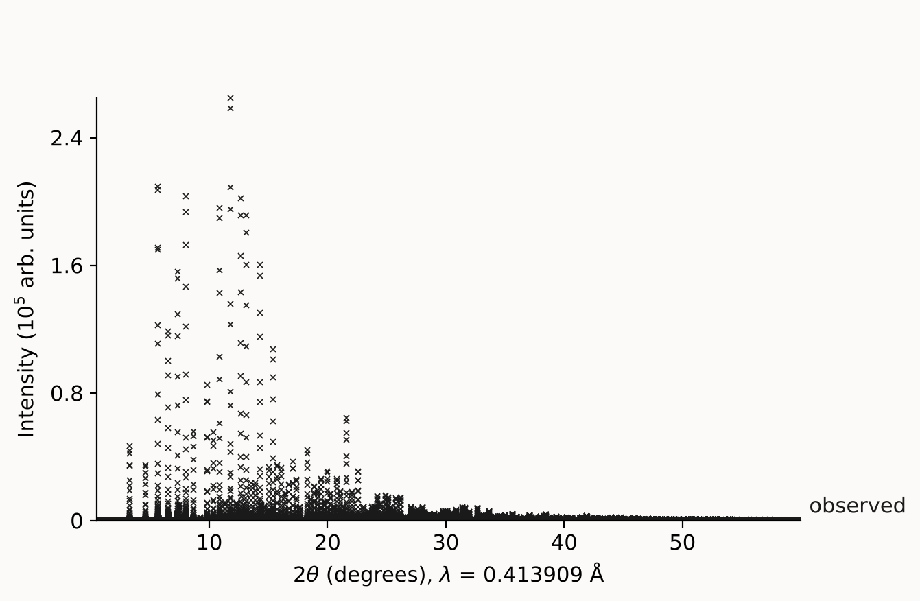
This is the 11-BM NAC pattern drawn with `data.plot(wavelength=0.4139090)`.
A `PatternData` carries no wavelength of its own.
The 2θ axis label names the radiation when something states it.
With `model=`, the instrument’s source states it.
Without a model, the anode and wavelength the file recorded in `metadata` do.
The label then reads `2θ (degrees), Cu Kα, λ = 1.54059 Å`.
An anode is named only where the source or the file states one, so a neutron or synchrotron source shows λ alone.
With neither, the label stays `2θ (degrees)`.
`wavelength=` replaces both.
A Q or d axis always needs `wavelength=`.
`model=` takes a `Refinement` and draws one row of reflection ticks per phase under the data.
The ticks sit at the model’s current positions, one set per emission line, and no fit runs.
They show whether a starting cell is close and the wavelength right.
A cell 1 % too large puts every fluorapatite tick visibly to the left of its peak.
`model=` also draws the background at its starting values, dashed, over the channels a fit would use.
Between the peaks it should run through the observed counts.
A background that is zero everywhere, as the default instrument’s is, is not drawn.
The rows sit below the data, so `model=` needs the linear intensity axis and refuses any other `y_scale`.
```python
import rietx as rx
from rietx.examples import examples_dir
folder = examples_dir()
data = rx.read_pattern(folder / "FAP.XRA")
ref = rx.Refinement(rx.Structure.from_cif(folder / "fluorapatite.cif"),
rx.Instrument.bragg_brentano(radiation="CuKa"))
fig = data.plot(model=ref, two_theta_range=(25, 40))
```
### Time-of-flight patterns
A time-of-flight pattern comes from a spallation neutron source such as ISIS, SNS or LANSCE.
The whole moderator spectrum reaches the specimen, and the reflections arrive in order of d-spacing.
This version reads such a pattern and refines none, because no flight-time forward model exists yet.
`Refinement`, `refine`, `MultiHistogramRefinement`, `refine_sequential`, `index_pattern`, `pick_peaks`, `diagnose`, `auto_background`, `PatternData.plot` and every other entry point that computes from a pattern raise on a flight-time axis or a `neutron_tof` instrument.
The message names the axis, its unit and the entry point.
With the bank’s calibration ([Time-of-flight bank](instrument.html.md#time-of-flight-bank)), the flight times convert to d-spacings.
### Checking a pattern before a fit
`diagnose(data, wavelength=...)` reads the pattern before any model exists and returns a `PatternDiagnostics`.
It reports how finely the peaks are sampled, whether the background carries a hump or an air-scatter rise, and where the signal runs out at either end.
It also reports which channels are dead, and whether the beam leaks Kβ or tungsten Lα.
Read `PatternDiagnostics.signal_cutoffs` first, because every other field is computed over the range it leaves.
[How to check a pattern before fitting](../guides/check.html.md) is the procedure.
[Pattern diagnostics](pattern-diagnostics.html.md) gives every field.
## Structure
`Structure` is a list of phases and nothing else.
`Structure.phases` may be empty.
A pattern whose phase is not yet known can still have its peaks picked and its cell indexed, under an instrument and a background.
A fit refuses an empty structure with `NoPhasesError`, because a background alone converges and would report `converged`.
`Structure.from_cif` reads a CIF or a magCIF, and `Structure.to_cif` writes one CIF block per phase.
A CIF states the crystal: the cell, the positions, occupancies and displacement parameters, and for a magnetic phase the moments and their group.
The phase scale and the broadening, extinction and preferred-orientation fields below are not CIF items.
`to_cif` does not write them, and `from_cif` returns them at their defaults.
`from_cif` reads an anisotropic displacement loop only when called with `aniso=True`, so reading a file never changes what a plan frees.
## Phase
`Phase` is one crystalline phase.
Its first five fields describe the crystal, and the rest describe what this specimen did to the peaks.
| Field | Type | Default | Meaning |
|---|---|---|---|
| `Phase.name` | `str` | required | a label, and the key an export writes |
| `Phase.space_group` | `str` | required | a Hermann-Mauguin symbol or a number as a string, resolved by gemmi; beside `symmetry_operations`, a label |
| `Phase.symmetry_operations` | `list[str]` or `None` | `None` | the operations as `x,y,z` triplets, for a group no symbol names in this cell |
| `Phase.cell` | `Cell` | required | the lattice parameters |
| `Phase.atoms` | `list[Atom]` | required | the asymmetric unit, at least one atom |
| `Phase.scale` | `Parameter` | 1.0, fixed, ≥ 0 | this phase’s share of the intensity |
| `Phase.lor_size` | `Parameter` | 0.0 deg, ≥ 0 | Lorentzian size broadening, as 1/cos θ |
| `Phase.lor_strain` | `Parameter` | 0.0 deg, ≥ 0 | Lorentzian strain broadening, as tan θ |
| `Phase.gauss_size` | `Parameter` | 0.0 deg², ≥ 0 | Gaussian size broadening, as 1/cos²θ |
| `Phase.gauss_strain` | `Parameter` | 0.0 deg², ≥ 0 | Gaussian strain broadening, as tan²θ |
| `Phase.magnetic_lor_size` | `Parameter` | 0.0 deg, ≥ 0 | extra Lorentzian size broadening of the magnetic intensity alone |
| `Phase.magnetic_lor_strain` | `Parameter` | 0.0 deg, ≥ 0 | extra Lorentzian strain broadening of the magnetic intensity alone |
| `Phase.extinction` | `Parameter` | 0.0 µm², fixed, ≥ 0 | primary extinction, the squared mosaic-block size D², [(5.12)](../theory/corrections.html.md#equation-corr-sabine); 0 is no correction |
| `Phase.preferred_orientation` | `PreferredOrientation` or `None` | `None` | March-Dollase preferred orientation, [(5.15)](../theory/corrections.html.md#equation-corr-md) |
| `Phase.texture` | `SphericalHarmonicTexture` or `None` | `None` | spherical-harmonics texture, [(5.17)](../theory/corrections.html.md#equation-corr-sh) |
| `Phase.microstrain` | `StephensStrain` or `None` | `None` | anisotropic strain, a width per hkl, [(6.7)](../theory/microstructure.html.md#equation-ms-sigma) |
| `Phase.particle_radius_um` | `float` or `None` | `None` | particle radius in µm for Brindley’s microabsorption correction, [(5.19)](../theory/corrections.html.md#equation-corr-brindley); never refined |
| `Phase.propagation_vector` | three rational strings, or None | `None` | a commensurate k on the conventional reciprocal cell, adding satellites at Q = H ± k, [(2.9)](../theory/peak-positions.html.md#equation-sat-position) |
| `Phase.magnetic_symmetry` | `MagneticSymmetry` or `None` | `None` | the magnetic space group, as its magCIF operator and centring loops, [(4.9)](../theory/intensities.html.md#equation-int-fmag) |
| `Phase.restraints` | `list` | `[]` | soft restraints on bonds, angles and values, [(9.17)](../theory/parameterisation.html.md#equation-par-restraint) |
| `Phase.floating_origin` | `"hold"`, `"centroid"` or `None` | `None` | what fixes the origin of a polar space group |
A phase can also carry rigid bodies over its own atoms.
That field belongs to the rigid-body technique, which is provisional by declaration ([Provisional by declaration](compatibility.html.md#provisional-by-declaration)); [Rigid bodies](../theory/parameterisation.html.md#rigid-bodies) gives the model.
A phase refuses three pairs of fields declared together.
`preferred_orientation` and `texture` are two models of one effect.
`propagation_vector` and `magnetic_symmetry` state one magnetic structure two ways.
A `microstrain` block and a free `lor_strain` refine the same column.
### Broadening
The four broadening terms are the specimen’s half of the peak width.
Gaussian variances add under convolution, and Lorentzian widths add, so the Gaussian pair is in deg² and the Lorentzian pair in deg.
Each term has the same angular shape as an instrument term, so one pattern cannot separate the two halves, and no shipped plan frees both.
`mccusker_default` frees the instrument widths and none of these four.
`lab_sample_refine` frees these four and none of the instrument’s.
[How to calibrate an instrument on a standard and reuse it](../guides/calibrate.html.md) gives the procedure.
`magnetic_lor_size` and `magnetic_lor_strain` broaden the magnetic component on top of the nuclear widths.
A non-zero value on a phase with no `magnetic_symmetry` is refused, and the parameter table lists the two only where `magnetic_symmetry` is declared.
`particle_radius_um` is a plain float, because the pattern cannot measure it.
Peak broadening measures the coherent domain.
That domain is smaller than the particle that Brindley’s absorption path runs through, and unrelated to it.
Take the radius from a micrograph or a particle-size measurement, or leave it `None`.
### Propagation vector
`propagation_vector` adds reflections, where every other phase field changes existing ones.
Declaring `("0", "0", "1/2")` puts a satellite at Q = H ± k beside every reciprocal-lattice point H of the phase.
A Le Bail or Pawley stage extracts intensity on the satellites, and a Rietveld stage contributes zero there, because no moment is stated.
That tests whether unindexed intensity in a neutron pattern indexes as satellites of a k, before any moment is stated.
The field enforces three rules.
- Each component is an exact rational. `"1/2"`, `Fraction(1, 2)` and `0.5` are stored as the same string, and a float that is not a rational of small denominator is refused. An incommensurate k needs superspace, which this version does not model.
- A k that is a reciprocal-lattice vector of the phase is k = 0 and is refused, because every satellite would land on a nuclear reflection. The test accounts for centring.
- `None` is off, and a phase with no k compiles to the reflection list it always had.
On an X-ray pattern the same declaration describes a superstructure reflection rather than magnetism.
The positions are identical, and nothing in the package can tell the two apart.
`magnetic_symmetry` and `Atom.moment` state the magnetic structure that a k only tests for.
Both default to `None`, which is off.
A moment needs `magnetic_symmetry` on its phase.
A moment outside the subspace the site’s magnetic symmetry allows is refused, and so is an atom carrying both a moment and an `aniso` block.
A free moment seeded at exactly zero is refused, because the magnetic intensity goes as m² and its derivative vanishes there.
### Symmetry operations
`symmetry_operations` states a space group that has no symbol in its cell.
A parent operation whose translation along a doubled axis is a half becomes a quarter in the child cell of a superstructure.
No Hermann-Mauguin symbol in any tabulated setting has a quarter in its operation list, but the group still has orbits, site multiplicities and systematic absences.
`None`, the default, resolves the operations from `space_group`.
With the list present, `space_group` is a label of one of two kinds.
- A bracketed label, such as `"Pm [unnamed in 2a,b,a+c]"`, names the nearest standard type, which does not generate this group. It requires the list, and no agreement between the two is checked.
- A plain symbol must generate exactly the listed operations. A disagreement is refused, because preferring either statement in silence is how a fit gets the wrong absences under a right-looking symbol.
A list that is not a group, with no identity or not closed under composition, is refused too.
Everything downstream reads the operations: site orbits and multiplicities, the Wyckoff constraint bases, systematic absences, the reflection list, the structure factor, the cell ties, the symmetry codes of bonds and angles, ZMV and weight fractions, and the GUI’s symmetry display.
`Structure.to_cif` writes the list as a `_space_group_symop_operation_xyz` loop.
`Structure.from_cif` reads a bracketed label beside such a loop back as the same list.
The GSAS, GSAS-II, TOPAS and FullProf writers refuse such a phase by name, because each of those formats states a group only as a symbol.
The cell’s metric constraints come from the tabulated group whose point group and lattice match the list, so they are exact.
Such a phase has no Wyckoff letters and never raises `SPACE_GROUP_SETTING_ASSUMED`.
`rietx.crystallography.magnetic.supercell.magnetic_supercell` builds such a phase and reports [`CHILD_GROUP_UNNAMED`](diagnostics-structures.html.md#child-group-unnamed) on the statement it returns.
### Floating origin
In a polar space group such as P 6₃ m c, P 4 m m, Cc or P 1, the whole structure can shift along the polar axis without changing any intensity.
`floating_origin` says what fixes the origin along each such direction.
- `"hold"` holds the first atom shift that moves along the direction, unless your own ties or holds already fix it. `Refinement.hold_floating_origin` sets this value on every phase whose group lets the origin float, and `Refinement.unhold` on the held shift sets the field back to `None`.
- `"centroid"` holds nothing. Each stage that can slide the phase gets one restraint per direction on a weighted centroid of the sites (Flack & Schwarzenbach, 1988), so every coordinate keeps an esd.
- `None` is off, and builds the table every earlier version built.
## Cell
`Cell` holds the six lattice parameters and applies no symmetry itself.
| Field | Type | Default | Meaning |
|---|---|---|---|
| `Cell.a`, `Cell.b`, `Cell.c` | `Parameter` | required | lengths in Å |
| `Cell.alpha`, `Cell.beta`, `Cell.gamma` | `Parameter` | required | angles in degrees |
The six carry no bounds of their own.
Store all six and let the space group decide which are independent.
The parameter table ties them by the space-group setting, which can differ from the crystal system.
An R lattice on rhombohedral axes needs a = b = c with the angles free, and monoclinic has three unique-axis choices.
A symmetry-fixed angle that disagrees with its symmetry is refused rather than snapped, because the table has no way to report a correction.
The CIF reader has one, so it corrects a small deviation and reports [`CIF_CELL_ANGLE_CORRECTED`](diagnostics-structures.html.md#cif-cell-angle-corrected).
`Cell.cubic` builds all six from one length, and `Cell.lengths_angles` returns the six values as a tuple.
## Atom
`Atom` is one site in the asymmetric unit.
| Field | Type | Default | Meaning |
|---|---|---|---|
| `Atom.label` | `str` | required | the site label, as a CIF spells it |
| `Atom.species` | `str` | required | the scattering species: `"La"`, `"B"`, `"Fe3+"` |
| `Atom.x`, `Atom.y`, `Atom.z` | `Parameter` | required | fractional coordinates |
| `Atom.occ` | `Parameter` | 1.0, at or above 0 | site occupancy; a refined value above 1 reports `OCCUPANCY_ABOVE_ONE` at `info` |
| `Atom.biso` | `Parameter` | 0.5 Ų, unbounded | isotropic displacement, B = 8π²U |
| `Atom.aniso` | `AnisoU` or `None` | `None` | anisotropic displacement as the CIF’s $U^{ij}$, [(4.5)](../theory/intensities.html.md#equation-int-dw-aniso) |
| `Atom.moment` | `Moment` or `None` | `None` | a magnetic moment in crystal-axis components, in μB, [(4.9)](../theory/intensities.html.md#equation-int-fmag); needs `Phase.magnetic_symmetry` |
| `Atom.disorder_assembly` | `str` or `None` | `None` | the CIF’s `_atom_site_disorder_assembly`: a cluster of disordered sites that is locally ordered |
| `Atom.disorder_group` | `str` or `None` | `None` | the CIF’s `_atom_site_disorder_group`: the sites of one assembly occupied together |
`species` is checked when the model compiles, so an unknown symbol fails with a crystallographic message rather than a schema error.
Coordinates do not refine as x, y and z.
The parameter table refines one shift per direction the site symmetry allows, and ties x, y and z to those shifts.
A fully fixed special position therefore has no free entry, and `vary=True` on one of its coordinates raises.
`Refinement.fix_special_positions` clears `vary` on every such coordinate and returns their names.
The [parameter map](parameters.html.md#atoms) gives the names of the shifts.
An atom has one displacement model.
With `aniso` set, `biso` is a record of the starting estimate, and asking to refine both raises.
`biso` has no bounds, as in FullProf, TOPAS and GSAS-II.
[`BISO_NEGATIVE`](diagnostics-refinement.html.md#biso-negative) and [`BISO_UNUSUALLY_LARGE`](diagnostics-refinement.html.md#biso-unusually-large) report a value outside the usual range.
The two disorder fields say which sites can be occupied at the same time.
Two sites in different groups of one assembly never are.
A group with a minus prefix marks a site disordered about a special position.
A site with no group is ordered and coexists with every other site.
`Structure.from_cif` reads both fields, and `Structure.to_cif` writes them back.
The fit does not read them, because the structure factor already weights each site by its occupancy.
The structure viewer reads them, to draw no bond between two alternatives.
```python
from rietx import Atom, Cell, Parameter, Phase, Structure
lab6 = Structure(phases=[Phase(
name="LaB6",
space_group="P m -3 m",
cell=Cell.cubic(4.15689, vary=True),
atoms=[
Atom(label="La", species="La", x=Parameter(value=0.0),
y=Parameter(value=0.0), z=Parameter(value=0.0)),
Atom(label="B", species="B", x=Parameter(value=0.19964),
y=Parameter(value=0.5), z=Parameter(value=0.5)),
],
)])
assert lab6.phases[0].cell.lengths_angles()[:3] == (4.15689, 4.15689, 4.15689)
```
## Optional blocks
Four blocks are absent by default: `Atom.aniso`, and `Phase.microstrain`, `Phase.preferred_orientation` and `Phase.texture`.
Each is opt-in because declaring one changes which parameters a plan frees, and reading a file must not do that in silence.
Each block at its identity values gives the same pattern as no block.
### Anisotropic displacement
`AnisoU` stores the six $U^{ij}$ of a CIF’s `_atom_site_aniso_U_ij` loop, in Ų.
`AnisoU.u11`, `AnisoU.u22` and `AnisoU.u33` are required, and `AnisoU.u12`, `AnisoU.u13` and `AnisoU.u23` default to 0.
`AnisoU.from_values` takes the six numbers in that order, and `AnisoU.values` returns them.
`AnisoU.isotropic` builds the tensor equivalent to a given $U_\mathrm{iso}$ in a given cell.
It is $U_\mathrm{iso}$ on the diagonal only when the reciprocal axes are orthogonal.
The components refine through the patterns the site symmetry allows, never one at a time.
`vary=True` on any component frees all of the site’s patterns, and `min` and `max` on a component have no effect.
A tensor outside the allowed subspace raises.
A tensor that stops being positive-definite raises [`ADP_NOT_POSITIVE_DEFINITE`](diagnostics-refinement.html.md#adp-not-positive-definite), because the Debye-Waller factor then diverges at high Q.
### Anisotropic strain
`StephensStrain` is Stephens’ anisotropic strain broadening.
It has fifteen coefficients, each named for the monomial $h^H k^K l^L$ it multiplies, in units of 10⁻¹² Å⁻⁴.
| H + K + L = 4, by shape | Fields |
|---|---|
| one index | `StephensStrain.s400`, `StephensStrain.s040`, `StephensStrain.s004` |
| three and one | `StephensStrain.s310`, `StephensStrain.s301`, `StephensStrain.s130`, `StephensStrain.s031`, `StephensStrain.s103`, `StephensStrain.s013` |
| two and two | `StephensStrain.s220`, `StephensStrain.s202`, `StephensStrain.s022` |
| two, one and one | `StephensStrain.s211`, `StephensStrain.s121`, `StephensStrain.s112` |
The coefficients multiply the literal monomials.
Some other programs fold the symmetry multiplicities in, so match a coefficient copied from another program by the width it produces, not by its name.
The space group’s operators decide which combinations are independent, and the coefficients refine through those.
`StephensStrain.from_values` and `StephensStrain.values` are the tuple interface.
`StephensStrain.isotropic` builds the block from one microstrain, in ppm of ΔM/M, and a cell.
It is the only legal starting point, because the width goes as a square root whose slope is unbounded at zero.
It sets `vary=True` by default.
Declaring the block locks `Phase.lor_strain`, whose column is the block’s isotropic direction.
σ²(M) ≥ 0 couples all fifteen coefficients, so it cannot be a bound.
The default solver holds it as a linear inequality.
Under `solver="trf"`, and in a joint fit, [`STEPHENS_STRAIN_NOT_POSITIVE`](diagnostics-refinement.html.md#stephens-strain-not-positive) reports where it fails.
### March-Dollase preferred orientation
`PreferredOrientation.axis` is the direction of preferred alignment as a fixed integer hkl, and `(0, 0, 0)` is refused.
`PreferredOrientation.r` is the one refinable number.
It defaults to 1.0, fixed, and r = 1 is no correction.
It is bounded below at `MARCH_R_MIN` (1e-6) and has no upper bound.
The March factor divides by r, so a stored lower bound at 0 is raised to `MARCH_R_MIN` when the object is built.
A stored upper bound is kept as written.
### Spherical-harmonics texture
`SphericalHarmonicTexture` is the general texture correction, for a texture with no single axis.
`SphericalHarmonicTexture.order` is the highest degree, even and at least 2.
`SphericalHarmonicTexture.coefficients` maps a term’s name to its `Parameter`.
The names follow GSAS-II’s C(l, n): `c4_0`, `c4_3`, `c4_neg3`.
Which terms exist depends on the Laue class.
A term you leave out is held at 0, and the parameter table makes an entry for every allowed term.
The table refuses a name the class does not allow, and an order with no allowed term, such as 2 for a cubic phase.
The coefficients have no bounds, because P ≥ 0 couples them all.
Every coefficient at 0 is no correction.
```python
from rietx.schemas.structure import SphericalHarmonicTexture
texture = SphericalHarmonicTexture(order=4)
assert texture.coefficients == {} # every term starts held at 0
```