# Derived quantities This page gives the quantities a fit computes from its refined parameters: interatomic distances and angles, each phase’s cell volume, and each phase’s crystallite size and microstrain in physical units, each with its esd. All three are fields of the `RefinementResult` a fit returns. [The refinement result](result.html.md) gives the rest of the result. Each esd is propagated through the parameter covariance, as [Esds of derived quantities](../theory/estimation.html.md#esds-of-derived-quantities) derives in equation [(8.7)](../theory/estimation.html.md#equation-est-derived). [About correlations and esds](../concepts/correlations.html.md#derived-quantities) explains why the whole covariance matters. ## Bonding geometry The IUCr guidelines rank the distances and angles above every R value. The two most important criteria for judging a refinement are the profile fit and the chemical sense of the structure [[McCusker *et al.*, 1999](../theory/references.html.md#id9)]. `RefinementResult.geometry` is a `GeometryTable` that carries the distances and angles. | Field | Is | Reads as | |---|---|---| | `GeometryTable.distances` | one `GeometryDistance` per neighbour | every asymmetric-unit atom’s whole environment, so the rows naming an atom count its coordination number and a bond between two sites is listed twice, once from each end | | `GeometryTable.bonds`, `GeometryTable.contacts` | the two halves of that list | split by `GeometryDistance.bonded` | | `GeometryTable.angles` | one `GeometryAngle` per pair of bonded neighbours | at every vertex, over that vertex’s complete bonded environment; a contact is never an arm | | `GeometryTable.bond_slack` | the slack added to the covalent-radius sum, in Å | 0.4 Å | | `GeometryTable.contact_max` | the listing radius for non-bonded contacts, in Å; bonds are found past it | 3.5 Å | | `GeometryTable.notes` | where coverage stopped | empty means nothing was bounded | A pair is bonded when its distance is at most the sum of the two covalent radii plus `GeometryTable.bond_slack`. A pair of two metals is always a contact, because a radius criterion is no evidence of a metal-metal bond. Past the slack a pair is still listed, as a contact, out to `GeometryTable.contact_max`. The guidelines ask for both kinds: “interatomic distances (both bonding and nonbonding) should be reasonable” [[McCusker *et al.*, 1999](../theory/references.html.md#id9)]. The slack and the search radius are conventions rather than physical constants, and the table records the values it used. Two limits write a note. Each atom keeps its 24 nearest contacts, and a note counts the contacts the cap dropped. A phase with more than 200 asymmetric-unit atoms is not searched, and a note names it. A row’s value is `GeometryDistance.distance` in ångströms, or `GeometryAngle.angle` in degrees. Each row names its atoms twice. The first naming uses the labels the structure carries: `GeometryDistance.atom_1` and `GeometryDistance.atom_2`, or `GeometryAngle.atom_1`, `GeometryAngle.atom_2` and `GeometryAngle.atom_3` with the vertex in the middle. The second uses indices into `Phase.atoms`: `GeometryDistance.atom_index_1`, `GeometryDistance.atom_index_2`, `GeometryAngle.atom_index_1`, `GeometryAngle.atom_index_2` and `GeometryAngle.atom_index_3`. `GeometryDistance.phase_index` and `GeometryAngle.phase_index` say which phase, in a multi-phase fit. `GeometryDistance.symmetry_2` is the CIF `n_klm` code of the image the second atom sits at. It resolves against the operation list the exported CIF writes beside it. The code holds a lattice shift of −4 to +4 along each axis, and an image that needs a larger one carries `None`. The distance and its esd are unaffected. `GeometryDistance.symmetry_1` is always `.`, the published position. So is `GeometryAngle.symmetry_2`, the vertex, while `GeometryAngle.symmetry_1` and `GeometryAngle.symmetry_3` code the two arms. A distance prints on one line, such as `Ca1–O5 2.3898(50) Å 5_565` from the fluorapatite tutorial fit. Geometry is computed for a Rietveld fit only. In Le Bail and Pawley mode `RefinementResult.geometry` is `None`, because the dummy atom those modes require is not a structure to measure. The table is computed when the fit closes. The covariance it needs comes from the final Jacobian, and the Jacobian is not stored. ### Esds of distances and angles `GeometryDistance.stderr` is propagated through the whole parameter covariance. The guidelines require the whole correlation matrix, and not only its diagonal, in the esd of any derived quantity [[McCusker *et al.*, 1999](../theory/references.html.md#id9)]. `GeometryDistance.stderr_diagonal` is the same propagation with the correlations between refined parameters set to zero. It is the number a reader combining the printed parameter esds in quadrature would get. It is reported so the difference can be seen, and it is never the answer. `GeometryAngle.stderr` and `GeometryAngle.stderr_diagonal` are the same pair for an angle, in degrees.  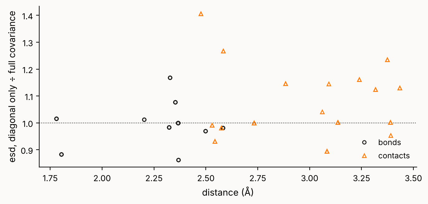Dropping the correlations is not a conservative approximation. The figure shows the 88 distances of an 11-BM NAC refinement under `mccusker_structural` (Rwp 0.0819), each as its diagonal-only esd over its full one. The ratio runs from 0.86 to 1.41, on both sides of one. So the diagonal-only number is sometimes too small and sometimes 40 % too large, and nothing in the row says which. The spread appears only once the coordinates refine. Under a plan that frees the cell and nothing structural, a cubic phase’s distances depend on one free parameter. The quadratic form then has one term, and the two esds agree to the last digit. The guideline is about correlation between coordinates, so a table quoted from a profile-only refinement shows no difference. ### Absent esds An esd is `None` when it cannot be measured. That is an absence, and it never means σ = 0. Four routes lead there: - The result has no covariance behind it. Any evaluate-only pass, a replay of a history node included, has distances and no esds at all. - Nothing free reaches the row. - Symmetry fixes the value, as for a fluorite Ca–F distance with the cell held, or a rutile O–Ti–O angle, which stays at exactly 90° however the one free coordinate moves. The variance then reaches zero by cancelling terms, and a variance below 1e-12 of the sum of those terms counts as zero. - The angle is within 2.6e-03° of 0° or 180°. Such an angle is a stationary point, where the linear propagation of [(8.7)](../theory/estimation.html.md#equation-est-derived) does not hold. The distance or angle itself is exact in all four cases. Only its uncertainty is withheld. ## Cell volume `RefinementResult.cell_volumes` holds one `CellVolume` per phase, in every mode, because a Le Bail cell is refined as surely as a Rietveld one. `CellVolume.phase_index` names the phase and `CellVolume.volume` is in ų. `CellVolume.stderr` goes through the covariance of the six cell entries, so a tie such as b = a and a correlation between a and c both reach it. On a cubic cell it is exactly 3a²σ(a). `CellVolume.stderr_diagonal` is the diagonal-only number, as for a distance. The four absences of a distance’s esd apply unchanged. The refinement CIF writes the volume with this esd. `RefinementResult.cell_volumes` is `None` on a result that did not come from a fit. ## Size and strain A refined profile width is a number of degrees, and a number of degrees does not transfer between instruments. The same 0.09° of 1/cosθ broadening is a coherent domain of about 410 Å on Mo Kα and about 880 Å on Cu Kα. `RefinementResult.microstructure` holds one `PhaseMicrostructure` per phase, in phase order. Each reads the four sample-broadening coefficients as the two quantities behind them. [Reading a width as a size](../theory/microstructure.html.md#reading-a-width-as-a-size) and [Reading a width as a strain](../theory/microstructure.html.md#reading-a-width-as-a-strain) state the two conversions as equations [(6.3)](../theory/microstructure.html.md#equation-ms-size-coefficient) and [(6.5)](../theory/microstructure.html.md#equation-ms-strain-coefficient). | Field | Is | Reads as | |---|---|---| | `PhaseMicrostructure.phase_index`, `PhaseMicrostructure.phase_name` | which phase the block is about | the index into `Structure.phases` and that phase’s `Phase.name`, so a block reads on its own in a multi-phase fit | | `PhaseMicrostructure.terms` | one `MicrostructureTerm` per sample coefficient | four rows (`lor_size`, `gauss_size`, `lor_strain`, `gauss_strain`), whether or not any of them refined; `PhaseMicrostructure.term` fetches one by coefficient name, such as `term("lor_size")` | | `MicrostructureTerm.kind` | `"size"` or `"strain"` | which conversion produced `MicrostructureTerm.value`: a coherent domain size in ångströms, or a dimensionless Δd/d | | `MicrostructureTerm.coefficient` | the refined coefficient | in its stored units, deg 2θ for the Lorentzian pair and deg² for the Gaussian variances, so a row can be checked against `RefinementResult.parameters` without converting anything | | `MicrostructureTerm.value`, `MicrostructureTerm.esd` | the reading and its esd | `None` for a cause that `MicrostructureTerm.unavailable` names | | `MicrostructureTerm.path` | the parameter it came from | such as `phases.0.lor_size`, so the row joins `RefinementResult.parameters` and any diagnostic’s `where` | | `PhaseMicrostructure.wavelength`, `PhaseMicrostructure.scherrer_k` | the two constants the size reading used | the source’s longest declared line, and the Scherrer K, so a size can be rescaled to another convention | | `PhaseMicrostructure.size_agreement`, `PhaseMicrostructure.strain_agreement` | the Gaussian reading divided by the Lorentzian one | 1 means the two independent columns describe one specimen; `None` when either reading is absent | | `PhaseMicrostructure.separable`, `PhaseMicrostructure.size_strain_collinearity` | whether size and strain are distinguishable over the range measured | read [Separating size from strain]() before quoting either number | `FitReport.microstructure` is a copy of the same list on the report, so a reader working from `Refinement.report()` need not go back to the result. The report adds one thing to its copy, the separability verdict. A coherent domain size is the length over which the lattice diffracts in phase. It is not a particle size and must not be reported as one. `Phase.particle_radius_um` is a different quantity for a different correction, the absorption path through a grain, and a particle is an aggregate of domains. A domain size is also not a two-figure number. K moves 10-20 % with crystallite shape, so `SCHERRER_K` = 0.9 is one convention among several. GSAS-II reads its size off the same FWHM with K = 1. FullProf reads it off the integral breadth, which for a pure Lorentzian is π/2 = 1.571 times the FWHM rietx uses. Quote the size as an order of magnitude, with the K the row carries. ### Separating size from strain Over a short 2θ range 1/cosθ and tanθ are nearly the same curve, so a fit can trade a size against a strain with no change in Rwp. That is the Williamson-Hall problem, and it is why a size is reported with `PhaseMicrostructure.separable` beside it. The verdict is the width trend’s own: `TrendAnalysis.separable` on the `"width"` observable, with `PhaseMicrostructure.size_strain_collinearity` carrying the correlation it was decided on. So the report holds one opinion about it. The report writes the verdict on its own copy, `FitReport.microstructure`. On `RefinementResult.microstructure` both fields stay `None`. On the report they are `None`, meaning no claim made, when Layer 1 abstained or no width trend was fitted. Where it says `False`, quote neither number alone. Refining one of the pair and holding the other does not help, because the answer then depends on which one was held. Measuring over a wider range does. ### Esds and absent readings Each reading is a function of exactly one refined coefficient, so its esd is that coefficient’s scaled by the derivative and nothing is dropped. For the Lorentzian pair the reading’s relative esd equals its coefficient’s. The Gaussian pair store a variance, whose square root is the width, so the reading’s relative esd is half its coefficient’s. A combined Gaussian-plus-Lorentzian size would be a function of two correlated columns, and is not reported. The two are read separately and compared through `PhaseMicrostructure.size_agreement` instead. `MicrostructureTerm.unavailable` names why a number is missing: | `unavailable` | What happened | |---|---| | `"at_zero"` | the coefficient is at its off state, where a size is infinite and a strain is a perfect lattice; true, and not a number to report. A phase whose widths were never refined says this in all four rows | | `"no_wavelength"` | the source declares no emission line, so no size can be read; a strain has no wavelength in it and never says this | | `"not_measured"` | the coefficient has no esd, so `MicrostructureTerm.value` stands and `MicrostructureTerm.esd` does not: the parameter was never freed, its column measured nothing, or the result came from `rietx.replay` | | `None` | nothing is missing | ### Size in a joint fit A joint fit shares the crystallite size and not the degrees it is read in. In a multi-histogram fit `MultiHistogramRefinement` normalises the size coefficients by wavelength. A Lorentzian size coefficient goes as λ and a Gaussian one as λ², while a strain coefficient does not depend on λ. The shared column is the coefficient at the first histogram’s wavelength, and each histogram’s own structure copy carries the value it needs. So the crystallite behind them is a single number, and the [`SIZE_NORMALISED_ACROSS_WAVELENGTHS`](diagnostics-series.html.md#size-normalised-across-wavelengths) diagnostic says so. Read a shared `phases.*.lor_size` as histogram 0’s coefficient, never as the number your second pattern shows.