The GUI panel by panel

The GUI: a first fit got one fit run and read. This chapter is the whole window: what each panel is for, and the handful of things about it that the screen cannot say about itself.

Read it beside the app rather than instead of it. Most controls carry their own explanation: a dotted underline means a definition is one click away, and the popover it opens is generated from the same help corpus Glossary is written from. What is written here is the part no tooltip can hold: why a control behaves as it does, and when you should reach for it.

The shape of the window

Two columns. The pattern on the left, a column of nine tabs on the right, and the console beneath them. Every panel is mounted at once, so a filter you typed, an edit you have not applied and a text buffer you are half way through all survive a look at another tab.

Split | Full in the header chooses how much window the panel column gets. It is a view choice and is not persisted; the panel widths you drag are, per project. Two panels want the room, and Full is for them: the Text document’s editable columns need about 550 px and the atom table about 470.

The header

Control	Does
the project chip	names the .rex, its data file, the point count, the intensity mode, and whether σ came from the file or from counting statistics
Rwp / GoF	the last run’s agreement; ⚠ not a fit yet appears beside it past an Rwp of 0.35
Open…	the import wizard, with the recent list in it
Split | Full	how much window the panel column takes
Simple | Advanced	whether rows nothing can free, bounds and transforms are shown
◐ ☀ ☾	theme: follow the system, light, dark
the run pill	the stage and its number while busy; the last status otherwise
Run / Cancel	start the plan; stop it between iterations
⌘K	every command, with the Python call it makes

There is no menu bar and no Save button, and neither is an omission. Settings persist on the verb. The moment you tick a box or drag a region it is written to the project, so there is nothing to save and nothing to lose on close. Save the project exists as a palette command for the one case that is not covered, which is writing out the settings file after an edit made from elsewhere.

The theme belongs to you and not to the project. It lives beside the recent list in the application’s own settings, so it follows you across projects, ports and browser profiles. It is also the one control that still works while a run is in flight, because it is not about the project.

The pattern

The left column is the measured points, the calculated pattern, the background, a band of reflection ticks, and the difference curve underneath.

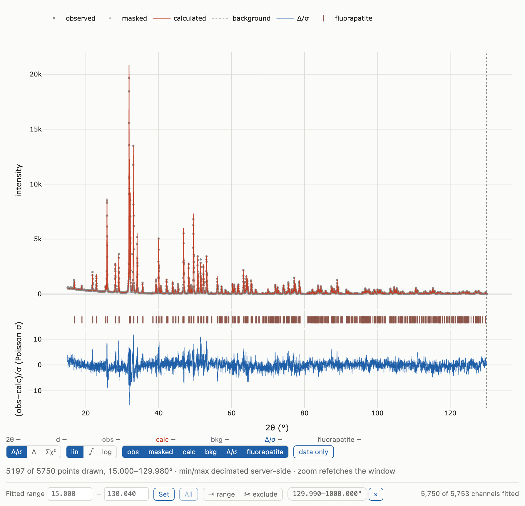
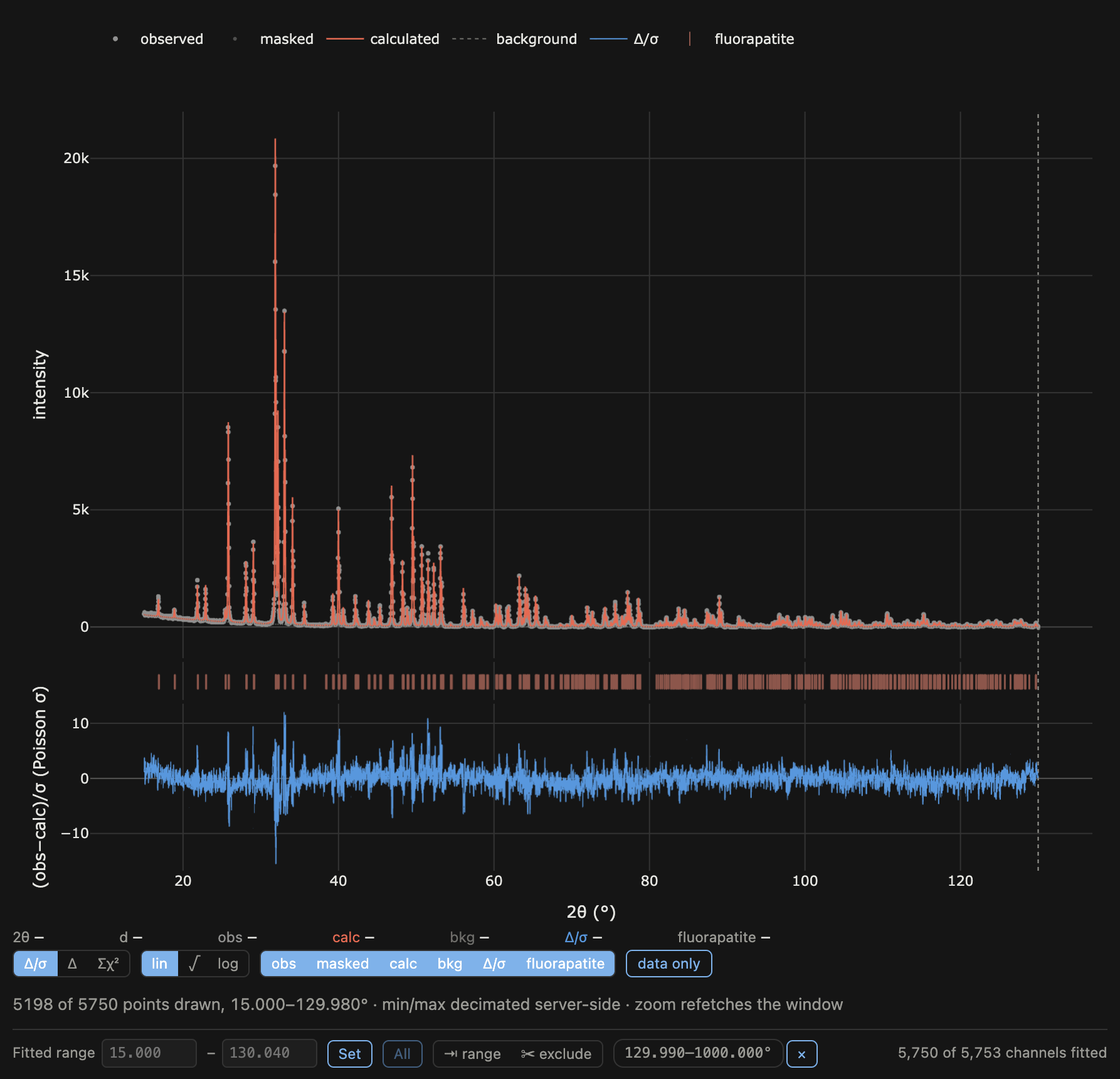
Reading under the pointer

There is no hover tooltip; a box that covered the data was worse than no box. What you get instead is the readout strip under the plot: a fixed set of slots that always shows 2θ and d, then one row per drawn curve, each label in that curve’s own colour, plus the nearest reflection of each phase as a signed offset. A slot empties to — when there is nothing under the pointer, so the plot above never resizes as you move. A solid vertical line marks where you are.

The strip follows what is drawn. Hide a curve and its row goes; press data only and the strip empties down to the measured points. That is correct behaviour.

The two kinds of knob

Only one kind changes the answer, and both sit under the same plot and look alike.

Drawing choices change the picture and nothing else. They are not persisted, so they reset with the session:

• the residual selector: Δ/σ, Δ, Σχ²;

• the intensity scale: lin, √, log;

• the per-curve visibility toggles, and data only.

Σχ² accumulates the weighted misfit from left to right, so a flat stretch is a region that cost nothing and a step is a region that cost a lot. A curve that is a staircase with one tall step tells you where to look in a way that no whole-pattern number can.

Protocol controls change what is fitted, move Rwp, and persist the moment you set them:

• the fitted range: two typed boxes, or the ⇥ range gesture;

• the excluded regions: a list of pills, or the ✂ exclude gesture;

• and beside them the count, N of M channels fitted, which makes the shaded band on the plot checkable.

Because settings persist immediately and curves only move on a run, the two can disagree, and the panel says so: the curves shown were fitted over a different set of channels — re-run.

The armed gestures

⇥ range and ✂ exclude are modes, not modifiers. Press one and the next drag on the plot sets a range or excludes a region instead of zooming; the cursor changes to say so, the peak gestures are suspended while it is armed, one selection disarms it, and Esc cancels.

They have to be modes because a region drag and a zoom drag are the same gesture at every distance. There is no radius at which the app could tell them apart. The peak gestures below are the opposite case, where the ambiguity is local and can be resolved by aim.

Zoom is a fetch rather than a crop: dragging refetches that 2θ window at full point budget, so zooming in gets you more points and not bigger pixels. Double-click returns the whole pattern, which the modebar’s home button also does less visibly. The view stays where you put it across a peak edit or a knob change.

Parameters

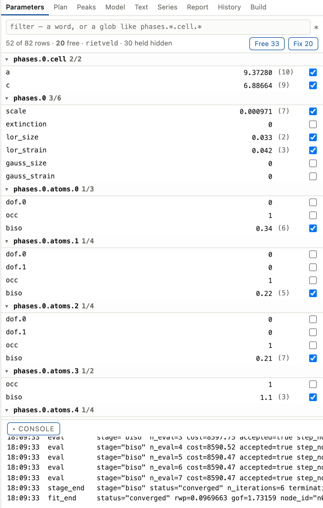
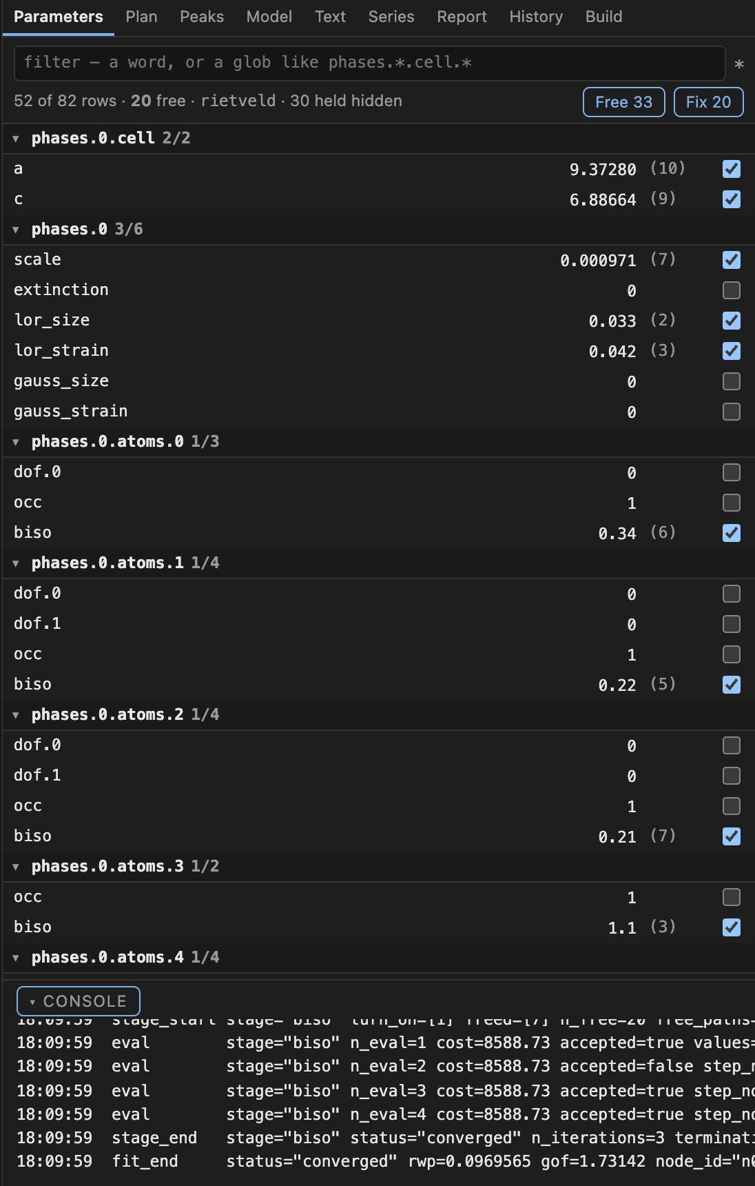
Every entry in the parameter table, one row each, with the control that frees it.

The filter box is the selection. Type a glob such as phases.*.cell.*, and the free and fix buttons act on the glob rather than on rows you have ticked. One glob is one set_vary call and therefore one history node, where a per-row multi-select would be one node per row. The count beside the box tells you how many rows the glob reaches before you act.

A row that cannot be freed has no checkbox at all. It carries a mark saying which of four reasons holds it: it is locked by symmetry, tied to another parameter, fixed by the intensity mode, or needs a held cell. Hover the mark for the reason in the package’s own words. Simple hides those rows along with bounds and transforms, and reports how many it hid; Advanced brings them back.

A typed value is compared against the value as displayed, so clicking into a cell showing 4.1568(2) and out again cannot truncate the parameter.

Plan

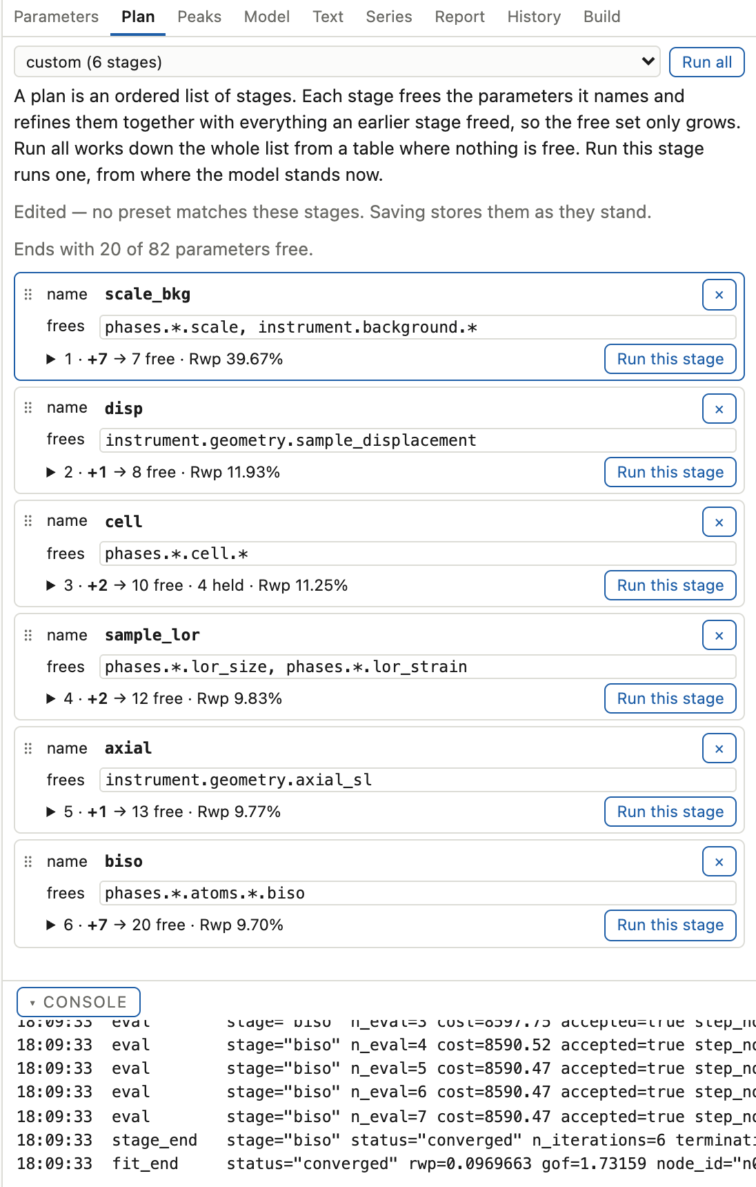
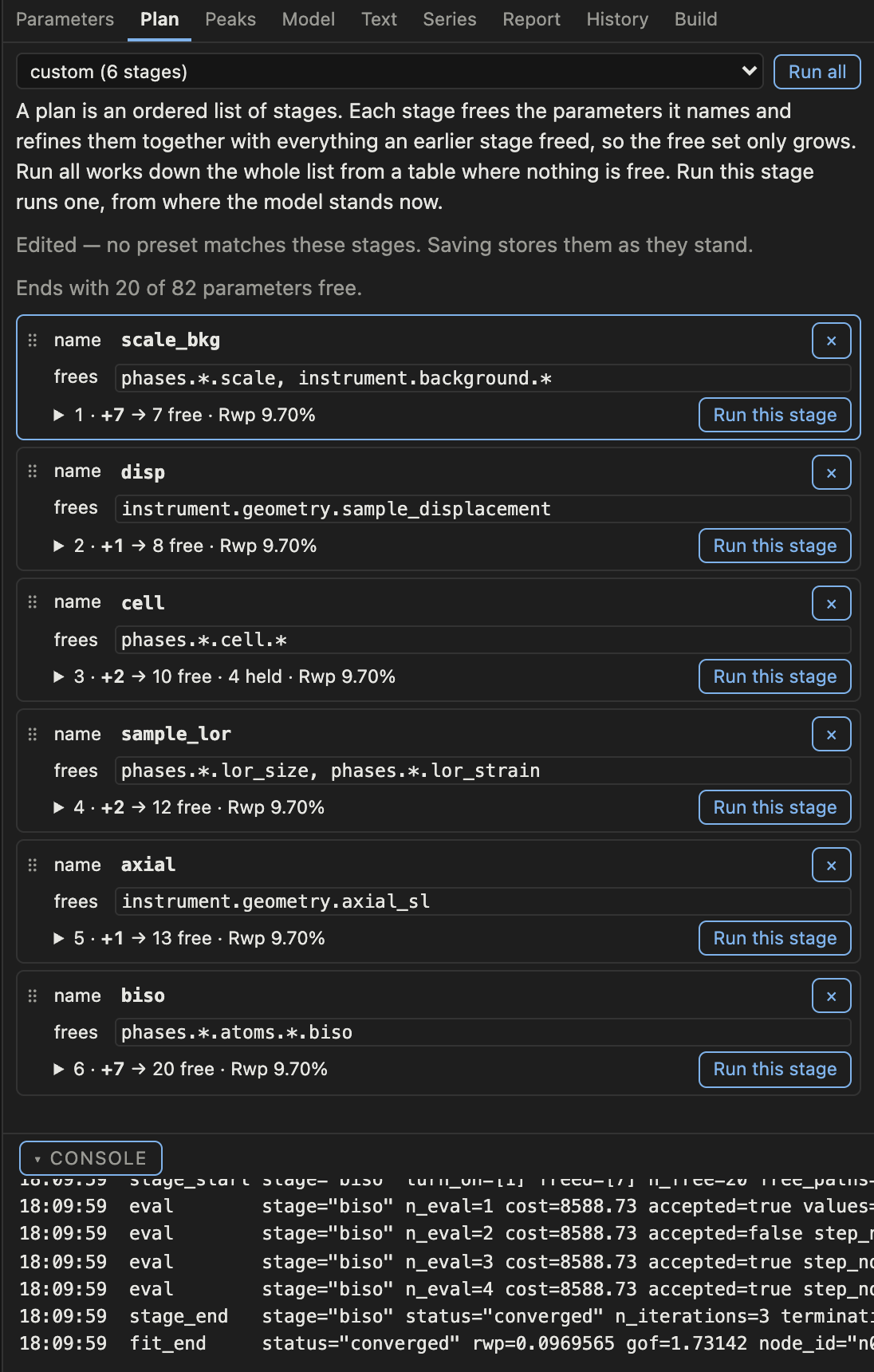
The stage list, and what each stage will actually do.

The panel resolves the plan against the real parameter table and shows, per stage, the paths its globs reach, which of them are newly freed, which are held and why, and the running count of free parameters. That resolution is the real verb and not a preview. It is the same call the fit makes, so the ties, the locks and the mode’s force-fixes shown are the ones you will get.

The two buttons do different things:

• Run all runs the plan from the start. A plan replaces the vary flags rather than continuing them, so a row you freed by hand that no stage names is dropped.

• Run this stage runs one stage from where you are, and keeps what you freed by hand.

A plan you have edited and not saved has no resolved facts and cannot be run, because the ladder describes the plan the server is holding.

Peaks

Two jobs: fitting individual lines, and finding a cell when you have no structure.

Picking lines

The plot becomes an editing surface while this tab is up, and prints its four gestures across the top whenever it is:

Gesture	Does	Typed route
click empty space	add a line	the panel’s 2θ box
drag a marker	move it	the Text pane’s 2theta column
shift-click	exclude a line from indexing	the row’s checkbox
right-click	remove it	the row’s ×

Every pointer verb has a typed twin. A pointer is not available to everyone, and a position typed to four decimals is not a position aimed at with a mouse.

A drag only moves a line when you are zoomed in far enough for the line to be visible. The grab radius is the smaller of 10 px and 1.5 fitted peak widths, so at a whole-pattern view a drag is always plotly’s zoom. Zoom first, then correct. Before that radius existed, a drag starting near a marker could move a line by degrees.

A line the fitter could not resolve is drawn differently rather than hidden, and the flag on its row says why. That is the fitter explaining the shape of a strong peak. A pasted position list is badged σ assumed, and its σ is a stated assumption rather than a property of your data.

Indexing

The Search controls disclosure is ProjectDoc.indexing as a form: which engines and crystal systems to search, centrings, a preset, bounds and budgets, and two editors for what you already know. Its vocabularies come from the build’s own capabilities, so a fourth engine would appear here with no new control written.

Three things to understand before reading an answer:

• The default is a bounded search. quick puts a ceiling on the whole run and streams a graded shortlist per crystal system as each finishes, so the first click gives an answer in bounded time. A low grade from a run that hit its ceiling means unconfirmed rather than bad, and the full search is one rerun away.

• A list with no high-confidence entry is a result. The whole module is built so that “the data cannot distinguish these” is sayable, and there is no setting that forces an answer.

• State what you already know. A prior cell or space group narrows the search honestly, where widening the tolerances does not.

Screen extinctions lives in a candidate’s expanded row: one row per extinction class, every space group in the class listed, and the reflections that refute it named. The teaching point is the package’s own. The extinction symbol is what a powder measures, and a single space group out of a class is a convention you choose rather than a measurement the table made.

Adopt turns a candidate into a Le Bail scaffold and flips the mode. The server’s own verdict enables it per row, and the badge does not.

Model

The structure and the instrument, and a 3D view of the cell.

The split explains why some edits feel different. If the parameter table has the path, the parameter table owns it: a cell edge, an occupancy, a Biso, a profile term go through the parameter routes, where the tie and lock rules already live. A species, a label, an atom added or removed, a geometry or a background family go as a whole validated model, because each changes what the table contains.

Two consequences you will meet:

• Coordinates are not typed as x, y, z. A site refines along the directions its symmetry allows, so the editor offers those; a fully fixed special position gets no coordinate control at all. Typing a whole position is possible, and the site answers. An unreachable one is refused, naming the directions it does allow and the nearest position they reach. It is never snapped, because snapping would move the atom to a different site than the one you asked for.

• An edit empties the plot until the next run. The curves described values the model no longer holds, so they are discarded rather than left to mislead. The workflow is edit, run, compare, and an empty plot there is the design.

The instrument form is three groups, Source, Geometry and Profile, and which group a field is in is a decision rather than its dot-path. The axial apertures are drawn with the profile they shape, and the zero shift beside the displacement it is refined against. U, V and W stand above X and Y. There is no Z; GSAS and FullProf spell these letters differently, so match the physics (size varies as 1/cos θ, strain as tan θ) and never the letter.

Changing a phase’s space group shows a preview of what the change would invalidate before it commits: incompatible values with their nearest allowed ones, coordinates that would be dropped, and the consequences a table diff cannot see, which are a setting change, an orbit collision, or the cell’s atom count doubling under a symbol with the same number of free parameters.

The 3D view

A third column of this panel, on by default, drawn by the server and rendered by the same plotly the pattern uses. Two modes: balls, and displacement ellipsoids. The projection is parallel and there is no axis box, so the cell’s own a, b, c edges are the frame of reference. Rotation is a free trackball, with buttons to view down a, b or c.

Two things here will mislead you if nobody says them:

• The bond threshold is a drawing threshold rather than chemistry. Bonds are drawn at a fraction of the sum of covalent radii, and no single value is right for both an ionic solid and an organic. LaB₆ at the default draws every La–B contact and looks like a cage; one turn of the slider down and the B₆ octahedron appears. It sits behind the drawing disclosure, and a first-time user needs it.

• The ellipsoids are a diagnostic. Their axes are refined quantities, so a background flexible enough to imitate the peaks arrives here as balloons, while improving Rwp. A non-positive-definite tensor arrives as a flat disc with the reason in its hover. Six ordinary-looking numbers in the parameter table are obvious in the picture.

The probability selector scales the ellipsoids. The × size factor beside it is a drawing multiplier and no ellipsoid stands above 100 %. A figure exported at a multiplier other than 1 is not an ORTEP-quotable surface, and the caption prints both numbers so it cannot be quoted as one by accident.

Element colours are chosen per phase rather than per element, so the same element can be drawn in two colours in two phases. The familiar assignments never move; the rest are separated against whatever else is in that phase.

Text

The whole project as one text document: settings, plan, and every parameter row, where @ frees a parameter and a bare value holds it. It is the fastest way to free thirty things at once, and the only panel where a rectangular selection (⌥-drag) makes sense. The format aligns its columns for that reason.

The normative description of the format is in The GUI as a text document and a wire. Two facts about using it belong here:

• There is no merge and no force-apply. If the project moved under your buffer, you re-read and re-apply. The reason is sharper than “merging is hard”: your stale document also carries the old value of every row you did not touch, so applying it anyway would silently revert them.

• Comments do not survive a re-render, because a document regenerated from the project has one authority and storing your comments would make two.

Series

The one panel whose subject is a method rather than a model. A series is N separate refinements chained by a warm start, and its trajectory is N answers in order. Reading it as one joint fit with a time axis through it is the mistake to avoid.

It runs under this project’s protocol: mode, plan, 2θ limits, excluded regions. The panel states those rather than offering them, because one protocol over N specimens is what makes their trajectories comparable.

Run it both ways once. direction="both" refines the chain forwards and backwards and flags the parameters the two passes disagree about. It is the only check that separates a measured trajectory from an ordering artefact, and a smooth curve is exactly what a poisoned chain produces. The panel banners the disagreement and draws the backward chain beside the forward one. Then decide whether you need to keep paying for the second pass.

The status column carries four chips, best learnt as two pairs. restaged and reseeded are both recoveries, the first still from the neighbour’s answer so the chain is unbroken, the second only from a cold start. hard means nothing rescued it but a warm attempt was still the best available, and unrecovered means it diverged on every attempt: it seeded no successor and joined no median. On the trajectory plot a ring marks a reseed and a cross marks an unrecovered point. They say opposite things: a ring is a good fit from a different starting model, a cross is not a measurement.

A series does not persist. Its patterns are staged uploads and its answer lives in the session, so closing the window loses the staged list. Say what you need from it before you close it.

Report

The FitReport rendered. The fit report is what the statements mean; five things about this panel will otherwise be misread.

• A suggestion with no Apply button is still a suggestion. Four of the action kinds are advice, and the note beside them is the deliverable. The background-flexibility pair is the case to watch: a more flexible background lowers Rwp while biasing displacement parameters up and scales down, so there is no honest one-click version.

• A greyed suggestion reading vetoed: is the engine agreeing with you and having already handled it. It looks like a refusal and is the opposite.

• “Could not rule out” is the headline. Where two explanations fit the misfit equally well, the report names both and caps its confidence rather than choosing. On the package’s own test case, applying a zero-shift correction to a fit whose cell was wrong improved Rwp from 21.6 % to 9.3 % by putting the error in the wrong parameter, and the report had said so in advance.

• The predicted Δχ² is one number for the whole report and it is not a bound. The panel prints it once, and it cannot be used to rank the suggestions.

• Applying a suggestion runs one stage, so it takes the same path the Plan panel’s per-stage Run takes and records one history node. Undo is a checkout, which throws the fitted curves away for the same reason an edit does.

History

Every state the refinement has passed through, drawn as a graph. What this panel changes is what you are free to try.

The rail is lanes, and a lane is where the tree divided. There are no named branches here and no moving refs. An edge runs down its lane and steps sideways in one row. Only a second parent is dashed, so a dashed line means “this rival strategy was folded in” and never “this is a merge”. With more lanes than the palette has hues a colour repeats, and that repeat is a collision you can see.

Select two nodes and the compare table reads path · a · b · Δ · Δ %, each side at its own family’s number of decimal places and the percentage taken against |a|. Only the Rwp badge is coloured for direction: a parameter difference has no good direction, and colouring one would be a claim.

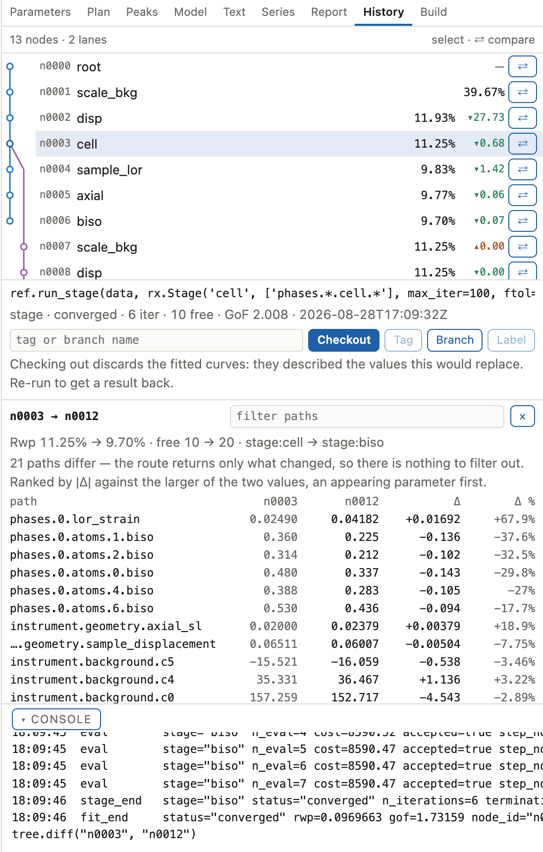
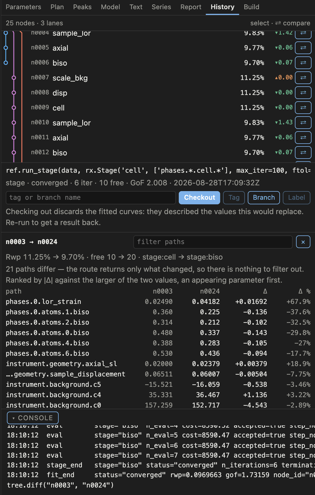
The picture above is the state this section is about: the plan was run, then run again from the cell node with a different strategy, and the two lineages sit side by side with a comparison of one node against the other underneath.

When to branch

A Rietveld refinement is a sequence of decisions that are hard to unmake. Free the wrong thing early and the fit slides into a minimum that looks fine and is wrong, and by the time the difference curve says so you have made ten more decisions on top of it.

Branching turns that into an experiment you can run twice:

• Before a decision you are not sure of, branch, try it, and compare against the state you left. Freeing anisotropic displacement parameters, adopting a candidate cell and turning on preferred orientation are all that kind of decision. The comparison is the point: a correction that improves Rwp while moving a cell by 1000 ppm has told you something, and you can only see it beside the other answer.

• When two explanations both fit, run both. The report will already have told you it could not separate them; a branch each is how you find out whether they disagree about anything you care about.

• Before anything irreversible in the model, such as a space-group change or a replaced structure, because a checkout restores the parameter count and not only the values.

Checkout, tag and annotate are all here, and every one of them is a node. The history is append-only, so exploring it cannot lose anything.

Build

What this build of the package can do, rendered from its own capabilities: backends and whether each optional dependency actually imports here, solvers, plans, modes, anodes and the pattern formats that can be opened. It is derived, so it cannot claim a feature the installed package does not have.

It also lists the panels the GUI plan still owes, which is currently none.