How a refinement works

A Rietveld refinement is one non-linear least-squares problem. The package computes a pattern from the model, compares it with the measurement point by point, and moves the free parameters to reduce the weighted sum of squares.

Almost everything that goes wrong is a correlation: two parameters change the calculated pattern in nearly the same way, so the data cannot tell them apart, and the solver splits the difference between them however the starting point happened to lean. This chapter is about which parameters those are and what the package does about it: how they are grouped, why the groups fight, and the three things you can do about it — order the refinement, tie two parameters together, or restrain a quantity you know. Reading the numbers is the numbers that come back.

The parameter groups

Every refinable quantity has a dot-path, and the paths group by what the parameter does to the pattern. Patterns, structures and instruments is the objects the paths address, field by field, and The parameter table is the path grammar and the table itself; this section is what each group does and why the groups fight.

Group	Paths	Changes	Angular signature
scale	phases.*.scale	total intensity of each phase	flat in Q
background	instrument.background.*	the pedestal under the peaks	smooth in 2θ
position corrections	instrument.zero_shift, instrument.geometry.sample_displacement, instrument.geometry.capillary_offset_along_beam, instrument.geometry.capillary_offset_across_beam	where every peak sits	constant, cos θ, sin 2θ, cos 2θ
cell	phases.*.cell.*	where each peak sits, through its d-spacing	tan θ
instrument profile	instrument.profile.u, .v, .w, .x, .y	peak widths and shape	Gaussian: w constant, v tan θ, u tan²θ. Lorentzian: x 1/cos θ, y tan θ
sample broadening	phases.*.gauss_size, phases.*.lor_size, phases.*.gauss_strain, phases.*.lor_strain	the specimen’s own width contribution	size 1/cos θ, strain tan θ
anisotropic strain	phases.*.microstrain.dof.*	width, per hkl rather than per θ	tan θ, scaled by direction
coordinates	phases.*.atoms.*.dof.*	relative peak intensities	none — it is an hkl effect
displacement	phases.*.atoms.*.biso, phases.*.atoms.*.adp.*	intensity falling off with Q	exp(−2B sin²θ/λ²)
occupancy	phases.*.atoms.*.occ	relative peak intensities	none
intensity corrections	phases.*.preferred_orientation.r, phases.*.extinction, instrument.geometry.surface_roughness.*	intensity, as a smooth or hkl-selective rescaling	various, all smooth in Q

Coordinates and occupancies refine differently from the rest, and it matters when you read a plan. A coordinate is not free in x, y and z; it is free along the directions its site symmetry allows, and ParameterTable wires one phases.*.atoms.*.dof.* entry per allowed direction and ties x, y and z to them. A fully fixed special position contributes no entries at all, so the glob is always safe to use, and setting vary=True on such a coordinate raises.

Anisotropic displacement parameters work the same way, through phases.*.atoms.*.adp.*, and so do the fifteen Stephens strain coefficients through phases.*.microstrain.dof.*. In each case the symmetry-allowed subspace is derived from the space-group operators, and a value outside it raises rather than being quietly symmetrised.

Why the groups correlate

Two parameters are hard to separate when their effects on the pattern have the same shape in 2θ. Over the whole range of a good dataset the shapes differ. Over a short range they do not, and that is where the trouble is.

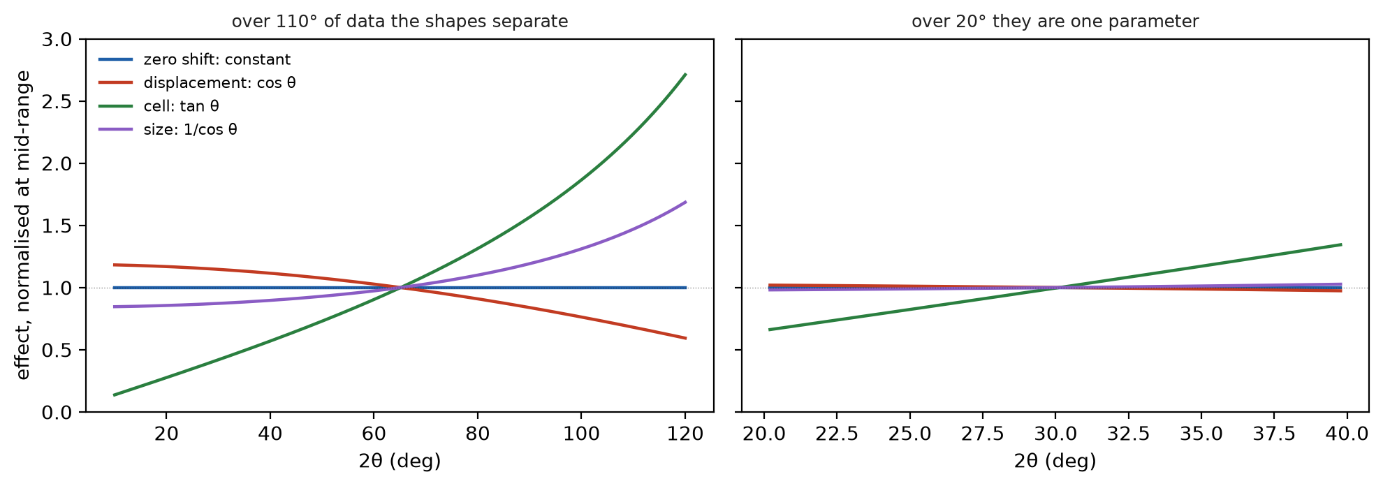
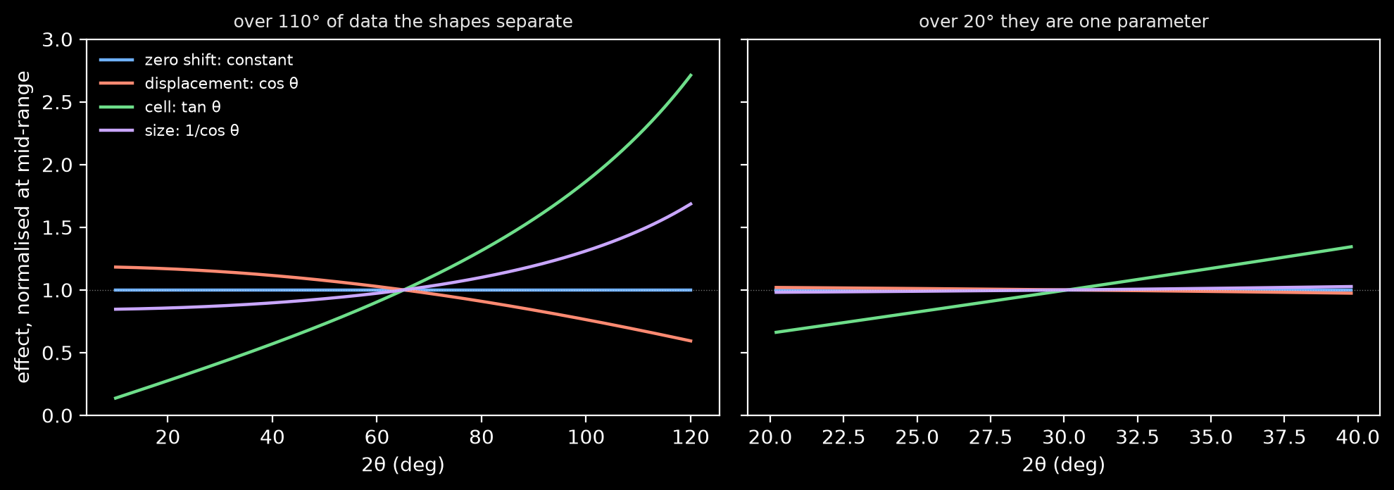
Each curve is normalised to 1 at the middle of its range, because separability is a question about shape and not about scale: two effects that differ only by a constant factor are one parameter, whatever their sizes. On the left, over 110° of data, the four are plainly different functions. On the right, over 20°, three of them are within a few per cent of each other and of a straight line. A refinement over that range reports four numbers and measures rather fewer.

Correlated group	Signatures	What goes wrong
zero shift · sample displacement · cell	constant · cos θ · tan θ	over a narrow 2θ range these three are collinear. A cell refined against a free zero shift on 20° of data is not measured.
zero shift · the two capillary offsets (Debye-Scherrer only)	constant · sin 2θ · cos 2θ	the same problem in the transmission geometry’s own shapes. Over 5-160° the three are separable; over 5-25° they are not, by a factor of about 4600 in the conditioning.
crystallite size · microstrain	1/cos θ · tan θ	the Williamson-Hall separation. Over a short range they are one parameter, not two.
scale · displacement · background · absorption · surface roughness · extinction	all smooth in Q	the big one. Every member lifts or depresses intensity smoothly with angle, so any of them can absorb any other.
preferred orientation · occupancy	both rescale specific hkl	an occupancy refined against uncorrected texture is a texture measurement.
overlapped intensities (Le Bail, Pawley)	identical	the sum is determined by the data; the split is not.

Two of those groups are worse than correlated. Capillary absorption is exactly a reparameterisation of the scale and the displacement parameters — the fit is identical with and without it — so Geometry.mu_r is computed from the specimen and never refined. Flat-plate absorption is 60 to 99 % absorbable, so Geometry.mu_t is also computed rather than refined; the part that is not absorbable does move Rwp, and a wrong thickness lands partly in the fit and partly in the displacement parameters.

Which position correction exists depends on the geometry. cos θ is the flat-plate specimen-displacement shape, so Geometry.sample_displacement and Geometry.sample_transparency are held fixed on anything that is not bragg_brentano. A capillary off the centre of the 2θ circle has its own pair, McCusker eq (4): Geometry.capillary_offset_along_beam carries the sin 2θ half and Geometry.capillary_offset_across_beam the cos 2θ half, they exist only on debye_scherrer, and both need Geometry.goniometer_radius_mm, which eq (4) divides by. Both default to 0 and fixed. At a synchrotron with a crystal analyser the paper says the displacement error is eliminated, so freeing them there measures nothing; a laboratory capillary or Guinier camera is where they belong.

The report knows this. Its position templates and the actions they map to are chosen by geometry, so a capillary fit is never told to refine a flat-plate aberration it cannot free.

Two rules follow, and they are the reason plans exist:

1. Do not free the second member of a group until the first is pinned by something outside the fit. This is what the lab_calibrate workflow is for: refining a certified standard with its cell held fixed is what decorrelates zero shift from displacement from cell, because the cell is supplied rather than fitted.

2. A correlation above 0.98 means you refined one parameter and reported two. The package raises HIGH_CORRELATION when that happens. The answer is almost never to widen the bounds. Fix one of the pair, extend the data range until the signatures separate, or — where chemistry says the two quantities are the same quantity — constrain them to each other.

Constraining parameters to each other

A constraint makes two parameters one: the dependent leaves the free vector and follows its source exactly, so the parameter count drops by one and the observation-to-parameter ratio rises. That is different from a restraint, which adds an observation (a bond length, say) with a weight and leaves the parameter count alone.

Use one where the data cannot separate two quantities and chemistry says they need not be separated. Two of the cases the guidelines [MVDC+99] recommend are available here: equal displacement parameters across atoms in the same environment, and occupancies that must sum to a known total. The third, rigid bodies, is not.

ref = rx.Refinement(structure, instrument)

# the three oxygens of one phosphate group refine as one B
ref.tie_equal(["phases.0.atoms.4.biso",
               "phases.0.atoms.5.biso",
               "phases.0.atoms.6.biso"])

# a mixed site: occupancies that sum to 1
ref.tie("phases.0.atoms.1.occ", "phases.0.atoms.0.occ", scale=-1.0, offset=1.0)

ref.untie("phases.0.atoms.*.biso")     # release them again

Refinement.tie_equal takes the same fnmatch globs as set_vary, and the first match in table order carries the freedom while the rest follow it; pass source to choose a different one. Refinement.tie is the general affine form, value = scale·source + offset, of which tie_equal is the scale=1, offset=0 case, and Refinement.untie releases them. Each verb records a history node, so a constrained refinement replays as one, and a project reopens with the constraint still in force.

A tie shows up in the parameter listing as a held row: refinable is false, held_because names the sources, and TieSpec.user is true for the ones you declared. The ties the space group creates — b following a in a tetragonal cell, a coordinate following its site-symmetry direction — read the same way with that flag false, and they cannot be released: symmetry outranks a user tie everywhere the two meet. The parameter table reads a held row field by field.

The verbs refuse rather than approximate. A locked parameter, an already-tied one, a source that is itself tied (which would make a chain), a target the current intensity mode force-fixes, and an implied value outside the target’s own bounds are all refused with the reason and the parameter holding it.

What a constraint buys, and how to check it was earned

Fluorapatite on a laboratory diffractometer, refined twice under one protocol — the second time with the three phosphate oxygens’ biso tied together:

	free	tied
free parameters	20	18
observations per parameter	287.5	319.4
Rwp	0.097307	0.097355
B(O5) / Ų	0.2763(1810)	0.4138(899)
B(O6) / Ų	0.5279(1911)	0.4138(899)
B(O7) / Ų	0.4149(1282)	0.4138(899)

The return is precision: the constrained esd is smaller than the best of the three free ones. Rwp is not the evidence and cannot be — it moved by 0.05 % of itself, which is what “the constraint costs no fit quality” looks like.

The check to run first is in the free column. Each of the three intervals contains the tied value, so the free refinement does not contradict the claim that these are one parameter. Where the free values disagree by more than their esds, the atoms are telling you they are not in the same environment, and tying them replaces a measurement with an assumption.

Restraining a distance or an angle

A restraint is the other half of the bargain. Where a constraint removes a parameter, a restraint adds an observation: a distance, an angle or a parameter value you know from chemistry, with an uncertainty attached, competing with the data on the same least-squares footing. Powder data lose information to overlap, and this is the standard way of putting some back [MVDC+99, Was63].

Three kinds, declared on Phase.restraints:

from rietx.schemas.structure import AngleRestraint, BondRestraint, ValueRestraint

bond = BondRestraint(atom_i=0, atom_j=1, target=1.87, sigma=0.02)
angle = AngleRestraint(atom_i=1, atom_j=0, atom_k=2, target_deg=109.47, sigma=1.5)
occupancy = ValueRestraint(path="phases.0.atoms.1.occ", target=1.0, sigma=0.01)

structure.phases[0].restraints = [bond, angle, occupancy]

Restraint	Names the quantity with	Target
BondRestraint	BondRestraint.atom_i and BondRestraint.atom_j	BondRestraint.target, in ångströms
AngleRestraint	AngleRestraint.atom_i, AngleRestraint.atom_j — the vertex — and AngleRestraint.atom_k	AngleRestraint.target_deg, in degrees
ValueRestraint	ValueRestraint.path, any dot-path in the model tree	ValueRestraint.target, in that parameter’s own unit

The atom fields are positional indices into Phase.atoms, the same convention the dot-paths use. All three kinds carry the same two numbers beside the target. BondRestraint.sigma, AngleRestraint.sigma and ValueRestraint.sigma are the uncertainty you are claiming, and that is what decides how hard the restraint pulls; BondRestraint.weight, AngleRestraint.weight and ValueRestraint.weight multiply the row on top of it and default to 1.

Each restraint contributes one residual row, √weight·(computed − target)/σ, appended after the data rows ((9.5)). The rows land in the covariance, so they tighten the esds of the parameters they touch, and they are excluded from Rwp, the Durbin-Watson statistic and the Bérar-Lelann inflation, because they are not measurements of this pattern. RefinementResult.restraints is what they report back, and Reading the numbers reads it.

A distance obeys periodic boundary conditions, so the second atom is taken at a symmetry image. BondRestraint.op_index selects the symmetry operation and BondRestraint.translation the lattice shift; AngleRestraint.op_index_i, AngleRestraint.translation_i, AngleRestraint.op_index_k and AngleRestraint.translation_k do the same for each arm of an angle. Leave them out and the minimum image is resolved once, at the stage’s starting coordinates, and frozen for that stage — the same discreteness rule the reflection list follows. Name the image explicitly whenever a coordinate is expected to move far enough to change which image is nearest.

Refinement plans

Because the groups correlate, freeing everything at once from a poor starting point walks into a local minimum that a staged release avoids. A fit here is therefore a plan: a list of stages, each freeing one group and running to convergence before the next group joins. Parameters stay free once freed, so each stage refines everything released so far.

RefinementPlan carries the presets, named for the job each does:

import rietx as rx

rx.RefinementPlan.mccusker_default()      # scale+bkg -> zero -> cell -> W -> U,V,X,Y
rx.RefinementPlan.mccusker_structural()   # ... then coordinates, displacement, PO
rx.RefinementPlan.lab_bragg_brentano()    # ... with sample displacement, Ka2, FCJ axial
rx.RefinementPlan.lab_calibrate()         # instrument calibration, certified cell HELD
rx.RefinementPlan.lab_sample_refine()     # sample against a frozen calibrated instrument
rx.RefinementPlan.profile_only()          # Le Bail
rx.RefinementPlan.pawley_default()        # Pawley

The two standard presets are one chain. mccusker_default stops after the widths; mccusker_structural continues into the structure:

        graph TD
  subgraph a ["mccusker_default"]
    A["scale + background"] --> B["zero shift"] --> C["cell"]
    C --> D["W, the constant width"] --> E["U, V, X, Y"]
  end
  subgraph b ["mccusker_structural adds"]
    F["coordinates"] --> G["displacement"] --> H["preferred orientation"]
    H --> I["extinction"] --> J["surface roughness"]
  end
  E --> F
    

Each box is a Stage. Every stage runs to convergence with everything above it still free.

Refinement.fit also takes a plan by name (plan="mccusker_default"). PLAN_INFO reports each preset’s title, description, modes and when to use it, so a program can offer the choice without hard-coding a list.

A plan is an ordinary object, so you can edit it:

plan = rx.RefinementPlan.mccusker_default()
plan.stages.append(rx.Stage("biso", ["phases.*.atoms.*.biso"]))
result = ref.fit(data, plan=plan)

Stage takes fnmatch globs over the dot-paths, which is why paths carry no brackets: fnmatch reads [..] as a character class rather than an index.

Running a refinement is the rest of the machinery: the plan registry a program reads instead of hard-coding this list, the other settings a Stage carries, and how to run, watch or stop a fit.

Relaxing the restraints as the model improves

Each restraint carries its own weight. A stage can scale all of them at once, which is how the guidelines [MVDC+99] ask restraints to be used: the refinement minimises S = S_y + c_w·S_G ((9.6)), and c_w “is set high at the beginning of a refinement when the structure is incomplete or only approximately correct” and is reduced “as the structural model improves”. Stage.restraint_weight_scale is that c_w, one number per stage.

import rietx as rx

coords = ["phases.*.atoms.*.dof.*"]
plan = rx.RefinementPlan(stages=[
    rx.Stage("scale_bkg", ["phases.*.scale", "instrument.background.*"]),
    rx.Stage("coords_stiff", coords, restraint_weight_scale=300.0),
    rx.Stage("coords_free", coords),          # back to 1.0, the default
])

The default is 1.0, which leaves the restraints exactly as they were declared. 0.0 silences them for a stage without removing their rows, so the row count the fit statistics exclude does not change part-way through a plan.

What this buys is a path. On a synthetic case whose data under-determines two oxygen sites, starting from a Zr–O distance of 3.73 Å for a 1.87 Å bond, the plan above lands the bond at 1.872 Å with the coordinates 0.001 rms from truth; the same three stages left at c_w = 1 throughout converge with that distance at 4.834 Å — the restraint 148σ in tension, Rwp 0.0393 against 0.0327.

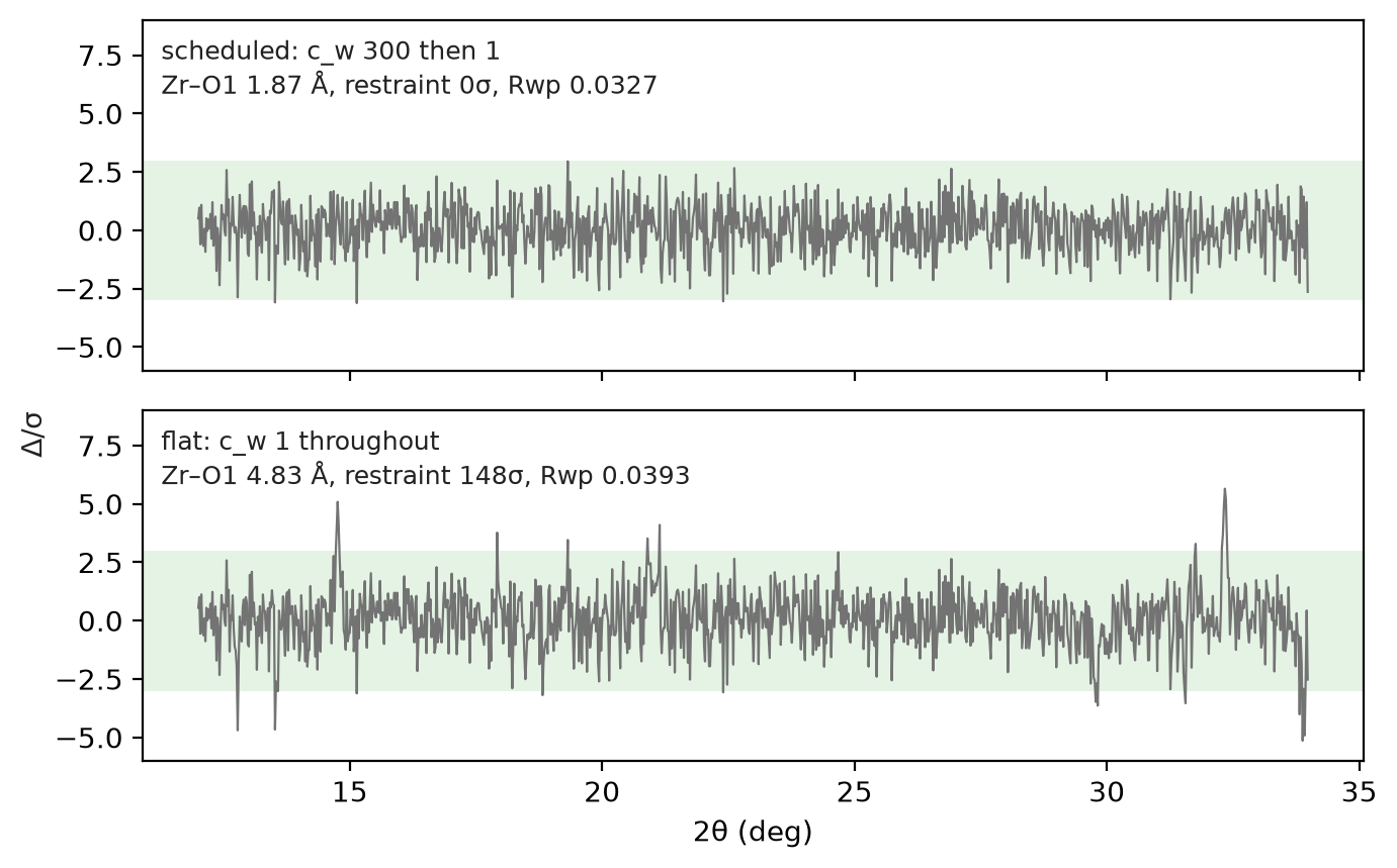
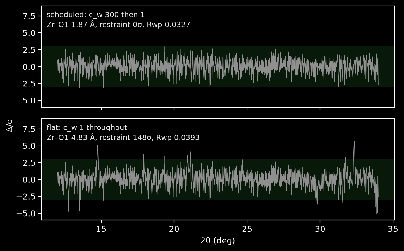
Both fits converged, on the same data, from the same start. The difference curves are the evidence a reader would normally reach for, and they are nearly the same curve. Read the restraint deviations instead: the failed fit is a slightly worse fit, not an announcement that a bond is 4.8 Å.

A stiff c_w makes a restraint more authoritative, not more correct. Where the chemistry assumed is wrong — the guidelines’ example is a tetrahedral site that is really octahedral — “the refinement will not progress satisfactorily”, and a higher weight makes that worse.

RestraintReport.weight_scale records the c_w a result was measured under, so a report always says which weight was insisting on its deviations. The deviations themselves are reported unscaled; Reading the numbers reads the rest of that object.

The order the presets encode

The backbone is the order McCusker et al. [MVDC+99] set out in the IUCr Rietveld refinement guidelines:

1. Background and scale first. The guidelines want good starting values for the background before the structure is touched, and the calculated pattern scaled to the observed one before anything is read off a difference plot.

2. Peak positions before everything else. The cell and the 2θ correction — the zero shift, plus sample displacement where the geometry has one — refine before the widths and before the structure. The guidelines put it flatly: unless the observed and calculated peak positions match, a Rietveld refinement cannot and will not work.

3. Then the widths, then the asymmetry. mccusker_default stops after the widths. lab_bragg_brentano and lab_calibrate continue in the guidelines’ order with a lines_axial stage — the FCJ axial-divergence ratios and the Kα2 weight — after them.

4. Then the structure: coordinates, then displacement parameters. The guidelines note that the scale, the occupancies and the displacement parameters are correlated with each other and are the parameters most sensitive to a background error, so they follow the positions rather than accompany them.

5. Everything free together at the end. Stages are cumulative for a reason the guidelines state explicitly: the esds are only correct when all parameters, profile and structural, are refined simultaneously. The last stage of every preset does that.

One departure: the guidelines suggest refining the heavier atoms’ positions before the lighter ones, and mccusker_structural frees every coordinate in one coordinates stage. Nothing here measures what the split would buy. If your structure has a large scattering contrast and a poor starting model, split that stage yourself — a plan is an ordinary object.

Three further ordering rules are this package’s own rather than the guidelines’:

• Widths last among the profile terms, and w before u, v, x, y. w is the constant term of the Gaussian width. Free the tan θ and 1/cos θ terms first and they absorb a constant offset, then fight it when w joins.

• Intensity-scaling corrections go last, after the structure has settled. Preferred orientation, extinction and surface roughness all rescale intensities as a function of Q — and so do the scale, the occupancies and the displacement parameters. Free a correction early and it eats intensity that belongs to the structure.

• Anisotropic strain is freed inside the sample-broadening stage, not after it. A Stephens block locks phases.*.lor_strain, because the isotropic direction of the block is identically that column. Deferring the block would leave the isotropic width unrefined until fifteen correlated coefficients turn on at once.

For agents

docs/AGENT_PROTOCOL.md §2 and §3 give the same order as an operating discipline, with the measured findings behind each rule — including what a Le Bail pass does that one fit call cannot.