Reading the numbers

A finished fit hands back a RefinementResult. This chapter is what is on it, and how to read each part: the agreement indices, the two structure R-factors, the distances and angles, what any restraints did, and the two counts that say whether the pattern could support the model at all. The refined parameter values themselves are the one part covered elsewhere, in The parameter table, because they are a view of the parameter table rather than a statistic about the fit.

The guidelines rank that evidence, and the ranking is not the one a table of R values suggests. The two most important criteria for judging a refinement are the fit of the calculated pattern to the observed one and the chemical sense of the structure [MVDC+99]. Rwp is half of the first.

Where a section here names a formula, Part 2 carries it as a numbered equation and this chapter links to it rather than restating it.

Fit statistics

RefinementResult.statistics is a Statistics object. The definitions follow Toby [Tob06], and Part 2 gives them as equation (8.2).

Field	Is	Reads as
Statistics.rwp	the weighted profile R-factor	how well the calculated pattern matches the measured one, weighted by the counting statistics. A fraction: 0.0932 is 9.3 %.
Statistics.rp	the unweighted profile R-factor	the same comparison with every point weighted equally, so strong peaks dominate it.
Statistics.rexp	the expected R-factor	the Rwp that perfect counting statistics alone would produce. It is a property of the data and the parameter count, not of the model.
Statistics.chi2	the reduced χ², Σw δ²/(N − P)	how far the fit is from statistical perfection. 1.0 means the residual is the size of the noise.
Statistics.gof	Rwp / Rexp	the square root of Statistics.chi2. Also called S or χ.
Statistics.rwp_background_subtracted	Rwp with the background removed from both patterns	the more meaningful figure when the background carries most of the raw intensity.
Statistics.durbin_watson	the serial-correlation statistic	≈ 2 means neighbouring residuals are independent. Far from 2 means the misfit is structured, whatever Rwp says.
Statistics.esd_inflation	the Bérar-Lelann factor	the amount the reported esds were multiplied by to account for that serial correlation. It has already been applied.
Statistics.n_points , Statistics.n_free_parameters	N and P	what makes the rest interpretable.

Statistics.chi2 is the reduced χ², not Σw δ². The two differ by a factor of N − P, which on a real pattern is several thousand.

The literature is not consistent about which of the two is called χ². The IUCr guidelines [MVDC+99] write χ² = Rwp/Rexp and say it should approach 1; that quantity is Statistics.gof here, and Statistics.chi2 is its square. Both conventions say the same thing about a fit — the naming follows Toby [Tob06] — but a number copied from a paper needs the convention copied with it.

Statistics.esd_inflation is conservative by construction. Perfectly white residuals still land near 1.51, because same-sign runs happen by chance, and lab data with unmodelled profile detail typically lands at 2 to 4. Treat it as an upper bound on the serial-correlation damage rather than as a measurement of it.

Structure agreement indices

Every field above measures the pattern. Two more measure the structure, and a journal will ask for at least one of them [MVDC+99]. They live on RefinementResult.phase_agreement, one PhaseAgreement row per phase, keyed by PhaseAgreement.name — the same name the phase carries everywhere else. Part 2 defines both as equation (8.3).

Field	Is	Reads as
PhaseAgreement.r_bragg	R_B, the Bragg-intensity R-factor	how well the model reproduces the integrated intensities I = m·F², m the multiplicity — rather than the profile. Written to a CIF as _refine_ls_R_I_factor.
PhaseAgreement.r_f	R_F, the structure-factor R-factor	the same comparison on the amplitude rather than the intensity, so it is the number a single-crystal R is directly comparable with. Written as _refine_ls_R_factor_all.
PhaseAgreement.n_reflections	how many reflections were summed	smaller than the phase’s reflection list whenever one falls off the Ewald sphere.

A joint multi-histogram fit reports them per histogram, on HistogramResult.phase_agreement: the partition is of one pattern’s counts, so there is no pooled value.

Both are biased towards the model you are testing. A powder pattern does not measure individual reflection intensities — overlapped peaks share their counts — so the “observed” intensity of each reflection is the observed pattern partitioned in proportion to the calculated one. A wrong model therefore receives the intensity it predicted, and both indices flatter it. That is the paper’s own warning, and it fixes what they are for: watching an R_B fall as you improve a model, not judging a model in isolation.

A trace phase’s R_B is not comparable with the major phase’s. Neither index is weighted — the sums count every reflection alike, whatever its counting statistics — so a reflection the fit barely constrains weighs as much as one that dominates it, and a minor phase’s windows sit under the major phase’s peaks, where the counts the major phase failed to describe are handed out too. Measured on the 11-BM NAC pattern with its 1.35 wt % CaF₂ impurity: NAC reads R_B 0.052 and the impurity 0.385, with the whole of the impurity’s misfit in four reflections at I(obs)/I(calc) ≈ 2.2 — every one of them under a strong NAC peak with a large positive residual. Read R_B beside the phase’s weight fraction, and treat a trace phase’s value as a question rather than a measurement.

Both are absent — an empty list — for a Le Bail or Pawley fit. There the intensities are the fit, so the partition would be compared against itself.

The bonding geometry

The other thing a journal asks for is the distances and angles, and the guidelines rank them above every R value: the two most important criteria for judging a refinement are the profile fit and the chemical sense of the structure [MVDC+99]. RefinementResult.geometry is a GeometryTable carrying them.

Field	Is	Reads as
GeometryTable.distances	one GeometryDistance per neighbour	every asymmetric-unit atom’s whole environment, so the number of rows naming an atom is its coordination number. A bond between two sites is therefore in the list twice, once from each end.
GeometryTable.bonds , GeometryTable.contacts	the two halves of that list	split by GeometryDistance.bonded: at most the two covalent radii plus GeometryTable.bond_slack, or beyond it out to GeometryTable.contact_max. The guidelines ask for both — “interatomic distances (both bonding and nonbonding) should be reasonable”.
GeometryTable.angles	one GeometryAngle per pair of bonded neighbours	at every vertex, over that vertex’s complete bonded environment. Contacts are not arms.
GeometryTable.notes	where coverage stopped	a per-atom contact cap or a phase too large to search. Empty means nothing was bounded.

A row’s value is GeometryDistance.distance in ångströms, or GeometryAngle.angle in degrees. Each names its atoms twice: as GeometryDistance.atom_1 and GeometryDistance.atom_2 — the labels the structure carries, with GeometryAngle.atom_1, GeometryAngle.atom_2 and GeometryAngle.atom_3 putting the vertex in the middle — and as GeometryDistance.atom_index_1, GeometryDistance.atom_index_2, GeometryAngle.atom_index_1, GeometryAngle.atom_index_2 and GeometryAngle.atom_index_3, which index Phase.atoms directly. GeometryDistance.phase_index and GeometryAngle.phase_index say which phase, in a multi-phase fit.

GeometryDistance.symmetry_2 is the CIF n_klm code of the image the second atom sits at, and resolves against the operation list the exported CIF writes beside it. GeometryDistance.symmetry_1 is always ., the published position; so is GeometryAngle.symmetry_2, the vertex, while GeometryAngle.symmetry_1 and GeometryAngle.symmetry_3 code the two arms.

The esd is the point

GeometryDistance.stderr is propagated through the whole parameter covariance, which is what the guidelines require of any derived quantity: “the whole correlation matrix, not just the diagonal elements, should be included in the calculation” [MVDC+99]. Part 2 gives the propagation as equation (8.6). GeometryDistance.stderr_diagonal is the same propagation with the refined parameters’ correlations zeroed — the number a reader combining the printed parameter esds in quadrature would get. It is carried so the difference is visible rather than asserted, and it is never the answer. GeometryAngle.stderr and GeometryAngle.stderr_diagonal are the same pair, in degrees.

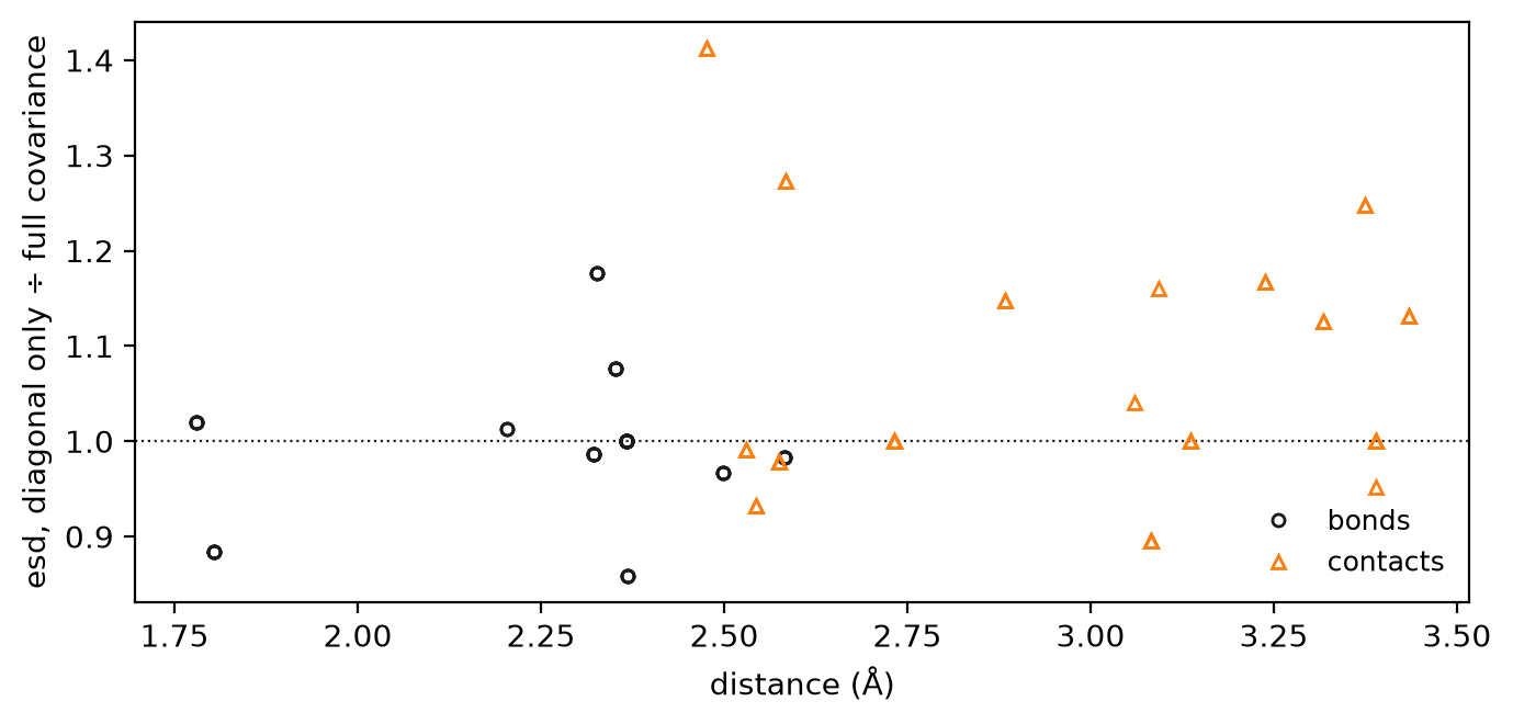
Dropping the correlations is not a conservative approximation, and that is the whole reason both numbers are reported. The figure is the 88 distances of an 11-BM NAC refinement under mccusker_structural (Rwp 0.0818), each plotted as its diagonal-only esd over its full one: the ratio runs from 0.86 to 1.41, on both sides of equality, so the cheap number is sometimes too small and sometimes 40 % too large, with nothing in the row to say which.

The spread appears only once the coordinates refine. Under a plan that frees the cell and nothing structural, a cubic phase’s distances depend on one free parameter, the quadratic form has one term, and the two esds agree to the last digit. Correlation between coordinates is what the guideline is about, which is also why a table quoted from a profile-only refinement has nothing to say here.

An esd is None when it cannot be measured, and None is absence, never σ = 0. Four routes lead there, and they mean the same thing. A result with no covariance behind it — any evaluate-only pass, a replay of a history node included — has distances and no esds at all. So does a row nothing free reaches. A row whose value is fixed by symmetry has no variance to report: a fluorite Ca–F distance with the cell held, or a rutile O–Ti–O angle, which stays at exactly 90° however the one free coordinate degree of freedom moves. And an angle at 0° or 180° is a stationary point, where the linearisation behind (8.6) does not hold at all. The distance or angle itself is exact in every one of the four; it is the uncertainty that is withheld.

Geometry is Rietveld-only. RefinementResult.geometry is None in Le Bail and Pawley mode, where the dummy atom the mode requires is not a structure to measure, and it is computed at the close of the fit rather than on demand: the covariance it needs is read off the final Jacobian, which is never stored.

How many observations there are

Statistics.n_points is the N the least-squares algorithm uses, and it is not the number of observations the pattern holds. Only the integrated intensities of individual reflections are unique observations [MVDC+99]; the profile steps across one peak are repeated measurements of the same number. The consequence is that the algorithm will refine far more parameters than the data support, without complaining, because its N runs into the thousands.

RefinementResult.data_support is a DataSupport object carrying the count that answers this. Part 2 states the correction it applies as equation (8.4).

Field	Is	Reads as
DataSupport.n_unique_reflections	reflections this pattern measured, summed over phases	one symmetry orbit is one reflection, and a Kα doublet’s second line is the same reflection measured again, not a second observation. A reflection counts when a fitted channel lies within half its own FWHM of its position, so an excluded region removes what sits under it and a peak half-measured at a range end still counts.
DataSupport.n_effective_observations	the same count corrected for overlap	each reflection contributes the fraction of its own area on which no overlapping reflection stands higher, so an isolated line is worth 1 and an exactly coincident pair is worth 1 between the two of them. A float, because a partly resolved pair is worth more than one and less than two.
DataSupport.n_structural_parameters	the free parameters the ratio is about	the atomic ones: coordinate DOFs, occupancies, Biso, ADP components. The cell, zero, profile, background, scale, preferred orientation and extinction are excluded — peak positions and shape determine those, not the intensities being counted.
DataSupport.observations_per_parameter	the raw count divided by the parameters	the upper bound on the ratio. None when no structural parameter is free, which is a profile-only stage, a Le Bail fit or a Pawley fit.
DataSupport.effective_observations_per_parameter	the effective count divided by the parameters	the number the guideline is about: at least three and preferably five [MVDC+99]. None on the same terms as the row above.

The complement of DataSupport.n_structural_parameters is Statistics.n_free_parameters minus it — the profile, background and cell parameters, which the same fit refined against the same pattern but which the peak positions pay for.

DataSupport.n_unique_reflections over-counts, on purpose. Two reflections at the same 2θ are one observation, and both are counted here. In a cubic cell that pair is common — (300) and (221) coincide exactly — so the raw count is an upper bound on the information, and the ratio built from it is optimistic. DataSupport.n_effective_observations is the corrected number, by the method of Altomare et al. [ACG+95], and the gap between the two is the pattern’s overlap.

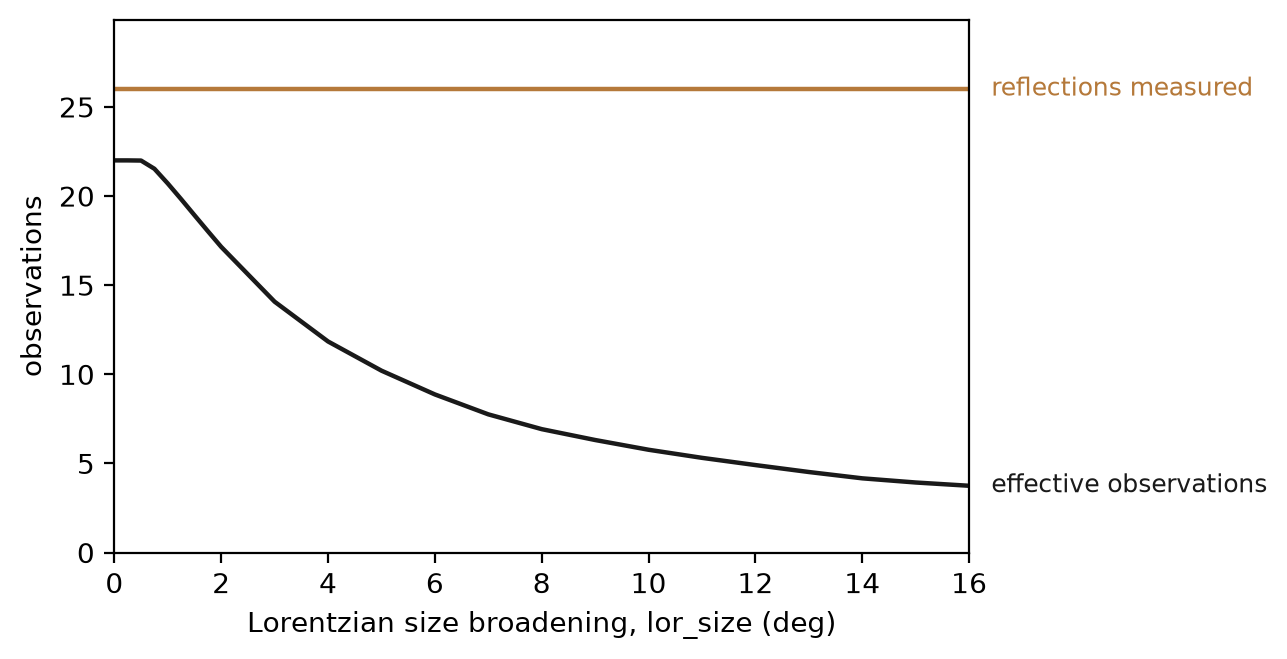
The figure is one Cu Kα LaB6 pattern over 15-140°, holding the cell and the reflection list fixed and widening the peaks with Lorentzian size broadening alone, so the overlap is the only thing that moves. Twenty-six reflections throughout; 22.0 effective observations while the lines are sharp, and 3.7 by the time the pattern is one hump. The raw count cannot see any of that, which is what makes it the wrong denominator for a parameter ratio.

The estimate is not a theorem. The paper says so, and the IUCr guidelines repeat it: the approach “may not have a rigorous basis”, and what it gives is a reasonable estimate of how many parameters the data will support. Two numbers a reader should have with it: the interval each reflection is judged over is ±2 FWHM, and the paper’s own check at ±4 FWHM lands 6.5 % lower on average, so the reported figure is a little generous.

Nothing here refuses anything. The number is evidence, read beside the fit rather than as a gate on it, and a ratio below three is a reason to hold parameters rather than a reason the fit is wrong. The sharper question — which parameter is unsupported, rather than how many the pattern can carry — is the identifiability evidence in the report. A ratio below five raises the DATA_SUPPORT_LOW diagnostic, as a warning below three and as information between three and five.

How finely the peaks were sampled

The other half of the question is about the experiment rather than the model. There should be at least five steps across the top of each peak, and generally not more than ten [MVDC+99]. Below five, the integrated intensity of that reflection was never measured, and no refinement afterwards recovers it.

PatternDiagnostics.steps_per_fwhm is that number: the median, over the pattern’s resolved peaks, of how many channels span the peak’s half-height width. PatternDiagnostics.n_peaks_measured says how many peaks the median was taken over. Both come from diagnose(data), which needs no model — so this is a question to ask of a file before refining it, and the answer does not change afterwards:

d = rx.diagnose(data)
print(d.steps_per_fwhm, "steps per FWHM over", d.n_peaks_measured, "peaks")

A refinement reports the same measurement on its fitted channels, as the PATTERN_UNDERSAMPLED diagnostic, and only when it falls below five. There is no code for the upper end of the band: oversampling costs beam time, not validity.

What the restraints did

If the fit carried soft restraints, RefinementResult.restraints is a RestraintReport, and on a restrained refinement it is the first thing to read, before Rwp. How a refinement works covers declaring them and scheduling their weight; this is the object that comes back.

Field	Is	Reads as
RestraintReport.rows	one RestraintRow per restraint	RestraintRow.computed against RestraintRow.target, with RestraintRow.deviation and RestraintRow.deviation_over_sigma the two ways of reading the gap — the second measured against the RestraintRow.sigma you declared, and RestraintRow.weight beside it. RestraintRow.kind, RestraintRow.atoms, RestraintRow.path and RestraintRow.phase_index say which restraint it was.
RestraintReport.restraint_chi2	Σ weight·(deviation/σ)²	the penalty term S_G of (9.6), at unit weight scale.
RestraintReport.weight_scale	the c_w the stage ran at	so the penalty the fit actually minimised is RestraintReport.weight_scale × RestraintReport.restraint_chi2.
RestraintReport.n_restraints	how many rows there were	the rows are in the covariance but out of Rwp, so this is not part of N.

The deviations themselves are always reported unscaled, because “is this restraint satisfied?” is a question about the geometry and c_w is a choice about how hard to insist on the answer. A row past three σ raises RESTRAINT_TENSION: the restraint and the data are pulling against each other, and one of them is wrong. A joint fit reports the same object per histogram on HistogramResult.restraints.

What the statistics cannot tell you

They measure agreement, not correctness. A background flexible enough to imitate the peaks biases displacement parameters up and phase fractions down while Rwp improves. Of the eight corrections shipped in v0.5, two provably cannot move Rwp, one moves it the wrong way when it is right, and the two largest accuracy wins are invisible in it.

That is what the report is for, and why a correction in this package ships with a record field or a diagnostic saying what it changed, rather than with an Rwp comparison as its evidence.

Diagnostics

RefinementResult.diagnostics is the channel for “your answer is wrong although Rwp is fine”. Each entry is a Diagnostic with a Diagnostic.code, a Diagnostic.level, a human-readable Diagnostic.message, a Diagnostic.suggestion, Diagnostic.where naming the parameter paths involved, and Diagnostic.value carrying the headline number where the diagnostic has one (a correlation’s ρ, an absorption’s block R²). None means “no single number”, not zero.

The codes are an open vocabulary, deliberately: a new correction ships with the diagnostic that states what it changed. Read them before the statistics, every time.