Patterns, structures and instruments

Three objects describe a refinement: the measured pattern, the crystal structure, and the instrument that recorded it. Files and projects says where each one comes from on disk. This chapter says what is inside them, so you can build one by hand, check what a reader handed you, or change one field without guessing what else moves.

Every number a fit can refine is a Parameter, and every Parameter has a dot-path. The parameter table is the table those paths address and how to read and edit a row of it; How a refinement works groups the paths by what they do to the pattern and explains which groups fight each other. This chapter is the objects those paths are built from.

The schemas reject what they cannot interpret. Every one of them forbids unknown fields, so a misspelled keyword is an error at construction rather than a setting that silently did nothing, and bounds are checked when the object is built rather than when the fit starts.

Every refinable number is a Parameter

Field	Type	Default	Meaning
Parameter.value	float	required	the current value, in Parameter.unit
Parameter.vary	bool	False	whether the least-squares problem is free in it
Parameter.min	float	-inf	inclusive lower bound
Parameter.max	float	inf	inclusive upper bound
Parameter.unit	str or None	None	a label, not a conversion: nothing rescales by it
Parameter.stderr	float or None	None	the esd, written by the fit
Parameter.transform	"identity", "softplus", "exp", "logit"	"identity"	internal reparameterisation, (9.2)
Parameter.expr	None	None	reserved, not implemented, and must stay None

value must lie within the bounds and min must not exceed max, both checked on construction. Infinite bounds survive a JSON round-trip as "Infinity", so an unbounded parameter is a legal thing to save.

from rietx import Parameter

a = Parameter(value=4.15689, min=4.0, max=4.3, vary=True, unit="A")
width = Parameter.positive(1e-3, vary=True, unit="deg^2")
assert width.transform == "softplus" and width.min == 0.0

Parameter.positive is the constructor for a quantity with no physical meaning below zero: a peak width, a scale, an absorption coefficient. It sets min=0.0 and the softplus transform, which keeps the optimiser away from the hard bound instead of letting it stall against it.

Warning

Softplus does not promise a strictly positive value. The internal variable maps to log(1 + exp(u)), which underflows to exactly 0.0 for u below about −745, so a min=0.0 softplus parameter can reach zero. That is harmless wherever zero is the off state, which is nearly everywhere in this package: a zero width is no broadening, a zero extinction coefficient is no extinction. It is a bug wherever the physics divides by the value, and such a parameter carries a real floor instead. PreferredOrientation.r is the one that does.

stderr is the one field a fit writes back. It is None on a parameter that was never free, and also on a free one whose esd could not be estimated; Reading the numbers explains what an absent esd means and how the fitted values are read back.

The pattern

PatternData is the measurement: two arrays of the same length, and what is known about their uncertainty.

Field	Type	Default	Meaning
PatternData.two_theta	list[float]	required	2θ in degrees, strictly increasing
PatternData.intensity	list[float]	required	measured intensity, same length
PatternData.sigma	list[float] or None	None	per-point esd from the file; None selects the Poisson fallback
PatternData.excluded_regions	list[tuple[float, float]]	[]	2θ intervals to leave out of the fit
PatternData.metadata	dict[str, str]	{}	what the reader found in the file header

Strictly increasing is enforced, not sorted for you. A file stored high to low is reversed by the reader, which reports that it did; a file whose 2θ column is not monotone at all is a refusal, because sorting it, concatenating it and splitting it are three different measurements. Files and projects has that rule and the four other places a reader may repair a file.

Five methods read the pattern out. PatternData.tt and PatternData.y are float64 numpy views of the two columns. PatternData.sig is the one that matters:

from rietx import PatternData

data = PatternData(two_theta=[10.0, 10.02, 10.04], intensity=[120.0, 480.0, 0.0])
assert list(data.sig().round(4)) == [10.9545, 21.9089, 1.0]

σ is a lookup and never a re-derivation. sig() returns the file’s sigma where the file had one and √max(y, 1) where it did not, and every weighted quantity in the package divides by the result: the objective (8.1), every renderer’s difference curve, both GUI windows. The Poisson fallback is correct for raw counts and wrong by √t for anything already divided by a counting time, so a reader that cannot establish the intensity scale withholds σ rather than inventing it. Reported esds of zero are floored, since a zero esd is an infinite weight on one channel. The floor is a thousandth of the column’s median positive esd, so it scales with the intensity’s units: the same pattern in counts or normalised to one is weighted the same.

PatternData.in_range_mask is the boolean mask that excluded_regions implies, and PatternData.crop returns a new pattern over a 2θ interval. Cropping and excluding are different acts: a cropped pattern has fewer points, an excluded region leaves the points in place and out of the residual. Prefer excluding, so the count that a statistic quotes still describes the file. A project records its excluded regions in its own document rather than in the pattern, for a reason Files and projects gives.

PatternData.plot draws the pattern as read, before any model exists. It forwards to rietx.viz.plots.plot_pattern, which is the data panel of RefinementResult.plot with nothing modelled in it: the same margins, gutter and intensity axis, and the same two_theta_range=, x_axis=/wavelength=, y_scale=, style= and title= keywords. The data and its fit are therefore one style, and a peak reaches the same height in both figures. An excluded region is shaded over channels that are still drawn, since they are measured counts the next fit will leave out. σ is not drawn, even when the file carried it.

from rietx import PatternData

data = PatternData(two_theta=[10.0, 10.02, 10.04, 10.06],
                   intensity=[120.0, 480.0, 200.0, 90.0],
                   excluded_regions=[(10.03, 10.05)])
fig = data.plot(title="as read")      # path="pattern.png" writes it
assert fig.get_axes()[0].get_title() == "as read"

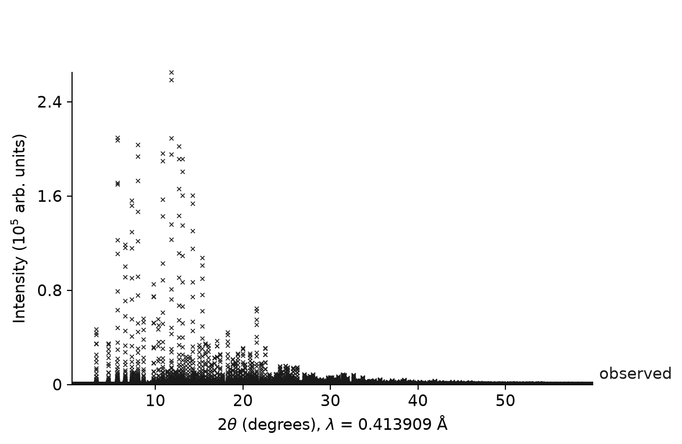
The figure is the 11-BM NAC pattern of the A first refinement, drawn with data.plot(wavelength=0.4139090) and no model. It is the quickstart’s fit figure with the fit taken out. A PatternData carries no wavelength, so λ on the 2θ axis, and a Q or d axis, need wavelength=.

Never subtract an estimated background from intensity. Hold it additively with BackgroundFixedPlusChebyshev or co-refine it under the smoothness penalty of BackgroundPSpline. Subtracting changes the counting statistics that sigma describes while leaving sigma alone.

diagnose(data, wavelength=...) reads the pattern before any model exists and returns a PatternDiagnostics: how finely the peaks were sampled, whether the background carries a hump or an air-scatter rise, where the signal runs out at either end, which channels are dead, and whether the beam is leaking Kβ or tungsten Lα. Reading the numbers documents every field. Run it on a file you have not seen before, and read signal_cutoffs first.

The structure

Structure is a list of phases and nothing else. Structure.phases carries at least one; Structure.from_cif reads one out of a CIF and Structure.to_cif writes it back.

Phase is one crystalline phase. Its first four fields describe the crystal and the rest describe what this specimen did to the peaks.

Field	Type	Default	Meaning
Phase.name	str	required	a label, and the key an export writes
Phase.space_group	str	required	Hermann-Mauguin symbol or a number as a string, resolved by gemmi, or, beside symmetry_operations, a label
Phase.symmetry_operations	list[str] or None	None	the phase’s symmetry operations as x,y,z triplets, for a group no symbol names in this cell
Phase.cell	Cell	required	lengths and angles
Phase.atoms	list[Atom]	required	the asymmetric unit, at least one
Phase.scale	Parameter	1.0, fixed, softplus	this phase’s contribution to the total intensity
Phase.lor_size	Parameter	0.0 deg, softplus	Lorentzian size broadening, 1/cos θ
Phase.lor_strain	Parameter	0.0 deg, softplus	Lorentzian strain broadening, tan θ
Phase.gauss_size	Parameter	0.0 deg², softplus	Gaussian size broadening, 1/cos²θ
Phase.gauss_strain	Parameter	0.0 deg², softplus	Gaussian strain broadening, tan²θ
Phase.extinction	Parameter	0.0, fixed, softplus	primary extinction (squared mosaic-block size), (5.12); 0 is E ≡ 1 exactly
Phase.preferred_orientation	PreferredOrientation or None	None	single-axis March-Dollase, (5.14)
Phase.microstrain	StephensStrain or None	None	anisotropic strain, width per hkl, (6.7)
Phase.particle_radius_um	float or None	None	Brindley microabsorption input, (5.17); a plain float, never refined
Phase.propagation_vector	tuple of three rational strings, or None	None	commensurate k on the conventional reciprocal cell; adds satellites at Q = H ± k, (2.8)
Phase.magnetic_symmetry	MagneticSymmetry or None	None	the magnetic space group as its magCIF operator and centring loops, (4.9); refused beside propagation_vector
Phase.restraints	list	[]	soft observational restraints, (9.11)

The four broadening terms are the sample half of the instrument ⊕ sample split. Gaussian variances add under convolution and Lorentzian widths add, so the two pairs carry different units: deg² for the Gaussian pair and deg for the Lorentzian one. Each term stacks on the instrument term with the same θ-dependence, so one pattern cannot separate the two halves, and no shipped plan frees both. mccusker_default frees the instrument widths and none of these four; lab_sample_refine frees these four and none of the instrument’s.

particle_radius_um cannot be obtained from the pattern at all, so it is a plain float rather than a Parameter. Profile broadening measures the coherent domain, which is smaller than and unrelated to the particle whose absorption path Brindley’s correction integrates over, and conflating the two is a standing error. Supply it from a micrograph or a particle-size measurement, or leave it None.

propagation_vector is the one field on a phase that adds reflections rather than changing what an existing one does. Declaring ("0", "0", "1/2") puts a second reflection at Q = H ± k beside every H of the phase’s reciprocal lattice; a Le Bail or Pawley stage then extracts intensity on those satellites and a Rietveld stage contributes exactly zero there, because this rung carries no moment and the nuclear model has nothing to say about the intensity of a magnetic satellite. That is the whole point: it lets you test whether unindexed intensity in a neutron pattern indexes as satellites of a k, without stating a single moment. Running a refinement covers the report arm that ranks candidates for you.

Three rules the field enforces rather than documents. Components are exact rationals, and any spelling ("1/2", Fraction(1, 2), 0.5, 0) is stored as the same canonical string, so a float that is not a rational of small denominator is refused by name: an incommensurate k is a superspace problem and is outside this rung. A k that is a reciprocal-lattice vector of this phase’s symmetry (the test is centring-aware) is k = 0 and is refused, because every satellite would land on a nuclear line and the reflection list would be exactly duplicated. And None is exactly off: a phase that declares no k compiles to the reflection list it always had, and every number the fit produces is unchanged.

On an X-ray histogram the same declaration means a superstructure reflection, not magnetism. The positions are identical; the inference is not, and nothing in the package can tell them apart for you.

magnetic_symmetry and Atom.moment are the other half of the same question, and they are the answer rather than the test: k on the nuclear cell with no moment asks whether the extra intensity indexes as satellites, and a magnetic space group with moments on the sites states the structure that produces it. Both default to None, which is exactly off, and the two are refused on one phase together with propagation_vector, because they are the same physics stated twice and nothing reconciles them. Running a refinement has the blocks, what refines and what the report says; Files and projects has how a magCIF, a TOPAS .inp or a FullProf .pcr gets one in, and how a magCIF or a TOPAS .inp takes it out again.

symmetry_operations is how a phase states a group that has no name in its cell, and the case is not exotic: a parent operation whose translation along a doubled axis is a half becomes a quarter in the child cell of a superstructure, and no Hermann-Mauguin symbol in any tabulated setting has a quarter in its operation list. The group is a perfectly good space group there: it has orbits, site multiplicities and systematic absences like any other, and the only thing it lacks is a symbol. Leave the field None (the default) and nothing changes: the operations are resolved from space_group exactly as they always were.

When the list is present, space_group is a label, and the rule is about labels. A bracketed label ("Pm [unnamed in 2a,b,a+c]") says that the symbol before the bracket is only the closest standard type and does not generate this group; it requires the list, and no agreement between the two is claimed or checked. A plain symbol beside a list must generate that list exactly, and a disagreement is refused rather than resolved in either direction: stating the symmetry two ways and being told when the two are not the same group is the point, and silently preferring one of them is how a fit ends up with the wrong absences under a right-looking symbol. A list that is not a group (no identity, or not closed under composition) is refused too.

Everything downstream reads the operations: site orbits and multiplicities, the Wyckoff constraint bases, systematic absences, the reflection list and its Laue multiplicities, the structure factor’s frozen operation subsets, the cell ties, the bond-and-angle symmetry codes, ZMV and the weight fractions, a magnetic phase’s reflection list, and the GUI’s symmetry facts and preview. The CIF export writes the list as a _space_group_symop_operation_xyz loop in its own order, and Structure.from_cif reads a bracketed label beside such a loop back as the same list. The GSAS, GSAS-II, TOPAS and FullProf project writers refuse such a phase by name, because each of those formats states a group only as a symbol. The cell’s metric constraints are the one thing an operation list cannot state directly, and they come from the tabulated group whose point group and lattice match the list, which are this group’s own, so they are exact rather than approximate. Two things such a phase does not get: a Wyckoff letter, and the SPACE_GROUP_SETTING_ASSUMED warning, both being properties of a tabulated setting. crystallography.magnetic.supercell.magnetic_supercell builds such a phase by itself and says so with a CHILD_GROUP_UNNAMED diagnostic on the statement it returns.

Cell holds six parameters and applies no symmetry itself.

Field	Type	Default	Meaning
Cell.a, Cell.b, Cell.c	Parameter	required	axis lengths in Å
Cell.alpha, Cell.beta, Cell.gamma	Parameter	required	angles in degrees

Store all six and let the space group decide which are independent. ParameterTable ties them from the space-group setting, which differs from the crystal system: an R lattice on rhombohedral axes needs a = b = c with the angles free, and monoclinic has three unique-axis choices. A symmetry-fixed angle that disagrees with its symmetry is refused rather than snapped, because the table has no channel in which to report a correction. The reader has one, so a small deviation is repaired at read and recorded; see Files and projects.

Cell.cubic builds all six from one length, and Cell.lengths_angles returns the six values as a tuple.

Atom is one site in the asymmetric unit.

Field	Type	Default	Meaning
Atom.label	str	required	the site label, as a CIF spells it
Atom.species	str	required	the scattering species: "La", "B", "Fe3+"
Atom.x, Atom.y, Atom.z	Parameter	required	fractional coordinates
Atom.occ	Parameter	1.0, in [0, 1.5]	site occupancy
Atom.biso	Parameter	0.5 Ų, in [0, 25]	isotropic displacement, B = 8π²·U
Atom.aniso	AnisoU or None	None	anisotropic displacement, CIF U^ij, (4.5)
Atom.moment	Moment or None	None	a magnetic moment in crystal-axis components, μ_B, (4.9); needs Phase.magnetic_symmetry beside it
Atom.disorder_assembly	str or None	None	the CIF’s _atom_site_disorder_assembly: a cluster of disordered sites that is locally ordered
Atom.disorder_group	str or None	None	the CIF’s _atom_site_disorder_group: the sites of one assembly occupied together; a minus prefix marks a site disordered about a special position

species is validated when the model compiles rather than when the object is built, so an unknown symbol fails with a crystallographic message instead of a schema error. Coordinates do not refine as x, y and z: the table wires one degree of freedom per direction the site symmetry allows and ties the three coordinates to those, so a fully fixed special position contributes no free entries at all and vary=True on such a coordinate raises. The parameter table has the paths and what a tied row looks like.

An atom has one displacement model. Set aniso and biso becomes an inert record of the starting estimate; asking to refine both raises rather than leaving a dead parameter in the vector.

The two disorder fields say which sites can be occupied at the same time. Two sites in different groups of one assembly never are. A site with no group is ordered and sits beside every other. structure_from_cif reads both from the file and Structure.to_cif writes them back. The fit does not read them: the structure factor already weights each site by its occupancy. The structure viewer does, to draw no bond between two alternatives.

from rietx import Atom, Cell, Parameter, Phase, Structure

lab6 = Structure(phases=[Phase(
    name="LaB6",
    space_group="P m -3 m",
    cell=Cell.cubic(4.15689, vary=True),
    atoms=[
        Atom(label="La", species="La", x=Parameter(value=0.0),
             y=Parameter(value=0.0), z=Parameter(value=0.0)),
        Atom(label="B", species="B", x=Parameter(value=0.19964),
             y=Parameter(value=0.5), z=Parameter(value=0.5)),
    ],
)])
assert lab6.phases[0].cell.lengths_angles()[:3] == (4.15689, 4.15689, 4.15689)

The optional blocks

Three fields take a block that is absent by default. Each is opt-in for the same reason: declaring one changes which parameters a plan will free, and reading a file must not do that silently.

AnisoU stores the six CIF U^ij components in Ų, the numbers a _atom_site_aniso_U_ij loop carries. AnisoU.u11, AnisoU.u22 and AnisoU.u33 are required and AnisoU.u12, AnisoU.u13, AnisoU.u23 default to zero. AnisoU.isotropic builds the tensor equivalent to a given U_iso for a cell, which is not U_iso on the diagonal unless the reciprocal axes are orthogonal. AnisoU.from_values takes the six numbers in order and AnisoU.values returns them. Components refine through the site-symmetry patterns rather than one at a time, so min and max on a component are inert and a tensor outside the allowed subspace raises.

StephensStrain is anisotropic strain broadening. Fifteen coefficients, each named for the monomial h^H k^K l^L it multiplies, in units of 10⁻¹² Å⁻⁴:

H+K+L = 4, by shape	Fields
one index	StephensStrain.s400, StephensStrain.s040, StephensStrain.s004
three and one	StephensStrain.s310, StephensStrain.s301, StephensStrain.s130, StephensStrain.s031, StephensStrain.s103, StephensStrain.s013
two and two	StephensStrain.s220, StephensStrain.s202, StephensStrain.s022
two and one and one	StephensStrain.s211, StephensStrain.s121, StephensStrain.s112

They multiply the literal monomials, where some other codes fold the symmetry multiplicities in, so a coefficient copied from another program has to be matched by the width it produces rather than by its name. Symmetry decides which are independent, and the space group’s own operators derive that set. StephensStrain.isotropic seeds the block from one strain in ppm of ΔM/M and a cell, and it is the only legal starting point, because the width goes as a square root whose slope is unbounded at zero. StephensStrain.from_values and StephensStrain.values are the tuple interface. Declaring the block locks Phase.lor_strain, whose column is identically the isotropic direction of the subspace.

PreferredOrientation is the March-Dollase correction: PreferredOrientation.axis is a fixed integer hkl and PreferredOrientation.r is the one refinable number, with r = 1 the identity.

The instrument

Instrument is everything about the measurement except the sample.

Field	Type	Default	Meaning
Instrument.source	Source or NeutronSource	required	the radiation, discriminated on kind
Instrument.geometry	Geometry	capillary, no aberrations	how the specimen sits in the beam
Instrument.zero_shift	Parameter	0.0 deg, in [−0.5, 0.5]	a constant 2θ offset, the one position error every geometry has
Instrument.profile	ProfileTCHZ	see below	the instrumental width function
Instrument.background	one of three	BackgroundChebyshev	the pedestal under the peaks
Instrument.extra_components	list[HumpComponent]	[] (off)	explicit broad peaks added on top of that pedestal

Four constructors build a plausible instrument, and the difference between them is which aberrations exist at all rather than which are switched on.

Constructor	Geometry	Radiation	Declares
Instrument.debye_scherrer	capillary	one wavelength you pass	polarization=0.99, optional capillary radius and µR
Instrument.bragg_brentano	flat plate, reflection	an anode name, Kα1 + Kα2	goniometer radius 217.5 mm, ka2_ratio=0.5, optional monochromator angle
Instrument.flat_plate_transmission	flat plate, transmission	an anode name, Kα1 by default	optional µt and thickness
Instrument.constant_wavelength_neutron	capillary	one wavelength, nuclear scattering	K pinned at 1, no dispersion, optional fwhm_deg width seed

from rietx import Instrument

synchrotron = Instrument.debye_scherrer(wavelength=0.4139090)
lab = Instrument.bragg_brentano(radiation="CuKa", monochromator_two_theta=26.6)
assert [line.wavelength.value for line in lab.source.lines] == [1.5405929,
                                                                1.5444274]
assert round(lab.source.polarization.value, 4) == 0.5557

That 26.6° is a Cu number rather than a property of graphite. The same crystal sits near 12.1° at Mo Kα, where K is 0.511 rather than 0.556, so compute it for the anode in use instead of copying the example.

Ask capabilities() for the anode names rather than trusting a list in prose.

The source

Field	Type	Default	Meaning
Source.lines	list[EmissionLine]	required	one entry per emission line, at least one
Source.polarization	Parameter	0.5	the fraction K of (5.1); 0.5 is an unpolarised beam
Source.dispersion	Dispersion or None	on	anomalous scattering, (4.8)
Source.harmonics	list[Harmonic]	empty	declared λ/n monochromator orders, refused on this radiation; see below
Source.kind	"xray_cw"	"xray_cw"	constant-wavelength X-rays

Source.primary_wavelength is the first line’s wavelength as a float, and it is the one every d-spacing is quoted against. Source.wavelength_parameters is the list of live wavelength Parameter objects, one per line, and is what code that needs to write a wavelength uses. NeutronSource.lines builds a fresh object per access, so a write through lines[i].wavelength lands on a throwaway there.

EmissionLine.wavelength is a Parameter in Å, defaulting to vary=False, and EmissionLine.weight is a refinable intensity relative to line 0. Line 0’s weight is structurally locked at 1, since it is degenerate with the phase scales. Each line diffracts at its own Bragg angle, so a doublet’s splitting grows with tan θ (2.5) and is never a fixed 2θ offset.

A bare number is still accepted where a wavelength Parameter is wanted, so EmissionLine(wavelength=1.5406) builds a fixed one and every instrument document written before this became a Parameter validates unchanged.

A refinable wavelength

EmissionLine.wavelength and NeutronSource.wavelength default to vary=False, and for a single histogram that default is a fence rather than a convention. Bragg’s law is (2.4), so the pattern measures λ/(2 sin θ) and fixes only the product of λ with a reciprocal cell. A free λ beside a free cell is an exactly flat direction, and freeing one is refused naming the degeneracy:

from rietx import Instrument
from rietx.params.vector import check_wavelength_freedom

instrument = Instrument.debye_scherrer(wavelength=0.4139090)
instrument.source.lines[0].wavelength.vary = True
try:
    check_wavelength_freedom(["instrument.source.lines.0.wavelength"],
                             n_wavelengths=1, n_histograms=1)
except ValueError as exc:
    assert "single-histogram" in str(exc)

Across several histograms of one specimen the degeneracy breaks, because they share one cell. A refinable wavelength states the rule in full and enforces it. The short version is to hold one wavelength and free at most N − 1, holding the one that belongs to the histogram that determines the cell.

This is EmissionLine.weight’s convention one rank up. In both cases one member of a set is pinned to fix a scale the data cannot set and the rest are free; what differs is where the set lives. A line weight’s scale lives inside one source, so line 0 is locked in the parameter table. A wavelength’s scale lives in the cell, which is shared across instruments, so no single instrument can count the set and the check sits where the joint problem is assembled.

Only line 0’s wavelength is ever refinable. Within one source the lines’ wavelength ratio is atomic physics: the tabulated Kα1/Kα2 pair traces to one NIST column for exactly this reason, and is known to about 20 ppm. So a secondary line’s wavelength is structurally locked, the way line 0’s weight is. The two locks are the same argument pointed in opposite directions. A weight is relative to something inside the source, and a wavelength is relative to something outside it.

One consequence follows. A monochromator’s second-order λ/2 harmonic cannot be modelled alongside a refining wavelength. Adding a second EmissionLine at λ/2 with its own weight models the harmonic at a fixed λ, and its wavelength would not follow line 0’s as that refines. Nothing here does that.

Dispersion is on by default. Dispersion.table names the tabulation and Dispersion.overrides takes measured f′, f″ pairs per element. Those are what you need near an absorption edge, where the table is wrong in principle rather than merely coarse. Setting dispersion=None declines the correction and reproduces the pre-v1.0 numbers exactly, and the fit says so with a diagnostic. It is the only correction in the package that needs no information a caller lacks, since the species and the wavelength are enough.

A neutron source

NeutronSource is the other arm of Instrument.source. It is a separate class rather than a flag on Source because almost every field of an X-ray source is meaningless for neutrons, and a class that has to explain which of its own fields are inert is worse than two classes.

Field	Type	Default	Meaning
NeutronSource.wavelength	Parameter	required	Å, vary=False; see A refinable wavelength
NeutronSource.harmonics	list[Harmonic]	empty	declared λ/n monochromator orders, see below
NeutronSource.kind	"neutron_cw"	"neutron_cw"	constant wavelength, the discriminator you write

Three read-only properties let code written for an X-ray source keep working. NeutronSource.lines is the fundamental followed by one line per declared harmonic. With none declared it is the single line, weight structurally 1, since with one line there is nothing for a relative weight to be relative to. NeutronSource.primary_wavelength is that wavelength as a float, and NeutronSource.wavelength_parameters is the live Parameter behind it, in a one-element list so a caller need not know which arm of the union it holds. That property is the one authority for writing a refined wavelength back: lines is a property here and a stored field on Source, so writing through lines[0].wavelength would land on a fresh object and the refined value would vanish at the next recompile. NeutronSource.polarization is 1.0 and refuses to be anything else, and NeutronSource.dispersion is always None.

Both of those last two are physics rather than simplifications:

• K = 1 is why no new correction code exists. Neutrons are not polarised by a monochromator the way the Thomson cross-section polarises X-rays, so the Lorentz-polarisation factor (5.1) collapses to the bare Lorentz factor 1/(sin²θ·cosθ), which is geometry and radiation-independent. K is force-fixed, so set_vary cannot free it. A free K would let the fit buy Rwp from a term the physics already knows.

• No anomalous dispersion. f′/f″ is an X-ray core-level effect. The neutron analogue is a complex, wavelength-dependent b near a nuclear resonance, which belongs to a handful of nuclides rather than to the source, so there is no field to set and DISPERSION_NEGLECTED stays quiet.

What actually changes in the calculation is the scattering amplitude, and only that. An X-ray form factor f(Q) falls off with angle because the electron cloud has spatial extent. A nucleus is a point scatterer on this scale, so b is independent of Q: one number per species instead of a five-Gaussian expansion, and it may be negative. Part 2 has the amplitude and its source.

Instrument.constant_wavelength_neutron is the constructor. It builds a capillary geometry, because a CW neutron diffractometer is a can of powder in a beam with detectors on a circle, so the cylindrical absorption correction and the capillary offsets apply unchanged.

from rietx import Instrument

bt1 = Instrument.constant_wavelength_neutron(wavelength=2.0780, fwhm_deg=0.3)
assert bt1.source.kind == "neutron_cw"
assert bt1.source.polarization.value == 1.0
assert bt1.source.dispersion is None

Pass fwhm_deg unless you have a reason not to. It seeds w alone, so the seeded profile is a flat Gaussian of fwhm_deg, with x left at its negligible default. The width you observed is the width you get, and it matters more here than on a lab X-ray: a neutron instrument’s lines are typically 0.2–0.5° where the ProfileTCHZ default is a synchrotron line of about 0.03°, and the per-stage evaluation windows are sized from the seed, so a 0.3° line started from the default is not found at all. The width function needs no neutron-specific code. The Caglioti law U·tan²θ + V·tanθ + W is the neutron resolution function, and the X-ray path is the borrower.

The width bounds do differ. ProfileTCHZ’s default box is sized for an X-ray line and caps w at 1 deg², a 1.0° FWHM, while a long-wavelength neutron line is wider: 1.10° on the ILL D1B Co₃O₄ tutorial set at λ = 2.52 Å, whose published model has U = 1.576, outside the default u bound. The default box stays, and the constructor refuses past it by name (WP-1312). The neutron preset builds that refusal’s escape for you: its profile is ProfileTCHZ.coarse, all five widths in TCHZ_BOUNDS_COARSE (u in [−0.5, 8], v in [−4, 4], w, x and y up to 8), so fwhm_deg may reach √8 ≈ 2.83° before it is refused by name. The cost of that ruling, said out loud: a bare wide width still refuses. ProfileTCHZ(u=1.576) raises, and the message names the two ways out, ProfileTCHZ.coarse(...) or an explicit Parameter(value, min, max) with your own bound. Every X-ray preset keeps the default box, so no X-ray fit’s search box moved.

from rietx.schemas.instrument import ProfileTCHZ

try:
    ProfileTCHZ(u=1.576)
except ValueError as refusal:
    assert "ProfileTCHZ.coarse" in str(refusal)
else:
    raise AssertionError("a bare wide width is refused")
d1b = ProfileTCHZ.coarse(u=1.576, v=-0.501, w=0.475)
assert d1b.u.max == 8.0 and d1b.w.max == 8.0

Two corrections are refused rather than ignored. surface_roughness is an X-ray effect: both models depress the low-angle intensity of a beam that penetrates microns, while a thermal neutron beam penetrates centimetres, so the correction has no regime here rather than a small coefficient. And a species this build has no tabulated scattering length for raises at compile naming the species, rather than contributing zero. A substituted zero would delete a site from the structure factor without changing the shape of anything.

λ/n monochromator harmonics

A crystal monochromator set to pass λ also reflects the higher orders of the same planes, so the beam carries a small λ/n component for every order that is not extinct (2.6). That component diffracts from the specimen too, and at a given 2θ it is diffracting from planes of spacing λ/(2n sin θ). So the harmonic’s peak from a given hkl sits at lower 2θ than the fundamental’s (2.7). Unmodelled, it is extra intensity in places the model puts none.

Declare it with Harmonic, on the source or through the constructor:

from rietx import Instrument
from rietx.schemas.instrument import Harmonic

bt1 = Instrument.constant_wavelength_neutron(
    wavelength=1.54040, fwhm_deg=0.3, harmonics=True)
assert [line.wavelength.value for line in bt1.source.lines] == [1.54040, 0.77020]
# a harmonic's λ is derived, so it is never free even when the fundamental is
assert [line.wavelength.vary for line in bt1.source.lines] == [False, False]

# general in n; True above is exactly [2]
thirds = Instrument.constant_wavelength_neutron(1.54040, harmonics=[2, 3])
assert len(thirds.source.lines) == 3
assert thirds.source.harmonics == [Harmonic(order=2), Harmonic(order=3)]

Field	Type	Default	Meaning
Harmonic.order	int ≥ 2	2	n in λ/n
Harmonic.weight	Parameter	0.01, fixed	intensity relative to line 0, like any emission line
Harmonic.wavelength_factor	float	derived	1/n, what the fundamental wavelength is multiplied by

Source.harmonics_supported and NeutronSource.harmonics_supported are class-level booleans saying whether that radiation accepts a declaration at all, False and True respectively. They are the one authority for the answer. The refusal below reads them, and so does RadiationCapability.harmonic_contamination, which is how the JSON surface reports it (Calling rietx from a program). Ask that rather than assuming, and never infer support from the presence of the harmonics field, which both classes have.

A harmonic is an emission line and not a phase. The usual workaround is an extra phase with a doubled lattice parameter, which gets the positions right and the intensities wrong: cell 2a has d′ = 2d, so λ diffracts from it where λ/2 diffracts from the real d, while its structure factors are those of a fictitious cell. A line at λ/n diffracts the same hkl list with the same |F|², because |F|² is a function of the reflection through sin θ/λ = 1/2d and not of the wavelength that reaches it. So positions and intensities come out together, and it costs one refinable number instead of a phase.

Empty is off, and off is exact: a source with no harmonic declared has the spectrum it always had, and reproduces every previously measured number bit for bit.

Three declarations are refused. order must be at least 2, since n = 1 is the fundamental and declaring it would be a second copy of line 0, degenerate with the phase scales. A repeated order is refused, because two lines at one wavelength with two weights on one physical component is a flat direction rather than a richer model. And harmonics are refused on an X-ray source: one f′ + i·f″ is frozen per phase and shared across every emission line, which is exact only while f is real, and λ against λ/2 is a 100 % wavelength change with absorption edges between them in general. capabilities().radiations reports which radiations accept them, read off the same attribute the refusal reads. On an X-ray source the route that does work is to declare the λ/n component as a plain EmissionLine with dispersion=None, where f = f₀ genuinely does serve both lines. The refusal’s message says so.

Whether a harmonic exists at all is arithmetic on the monochromator, and not something to discover from a fit. Cu(311) doubles to the allowed (622), so the second order passes; a diamond-structure crystal cut on all-odd indices cancels its own second order exactly. Part 2 has both.

Time-of-flight is not this

Everything here is constant wavelength. A time-of-flight instrument spans a range of wavelengths across several detector banks, which changes the profile function, the intensity corrections and the number of histograms at once, and the thermal scattering-length table cannot give b(λ) for a resonant absorber. capabilities().radiations is the list of what this build actually accepts.

The geometry

Geometry.kind selects one of "debye_scherrer", "bragg_brentano" and "flat_plate_transmission", and it decides which of the other fields are meaningful. A field that belongs to another geometry is refused rather than ignored.

Every geometry:

Field	Type	Default	Meaning
Geometry.kind	literal	"debye_scherrer"	which of the three geometries
Geometry.goniometer_radius_mm	float or None	None	R in mm; required for bragg_brentano, and what (2.14) divides by
Geometry.axial_sl, Geometry.axial_hl	Parameter	0.0	Finger-Cox-Jephcoat axial divergence: sample and detector half-lengths over R
Geometry.packing_fraction	float	0.6	solid fraction of the specimen, an absorption estimator input

A capillary, kind="debye_scherrer":

Field	Type	Default	Meaning
Geometry.capillary_offset_along_beam	Parameter	0.0 mm	the sin 2θ half of (2.14), positive downstream
Geometry.capillary_offset_across_beam	Parameter	0.0 mm	the cos 2θ half, positive toward increasing 2θ
Geometry.mu_r	float or None	None	µ·R of the packed specimen, (5.5); 0.0 is off exactly
Geometry.capillary_radius_mm	float or None	None	bore radius in mm, an estimator input for µR

A flat plate, kind="bragg_brentano" or kind="flat_plate_transmission":

Field	Type	Default	Meaning
Geometry.sample_displacement	Parameter	0.0 mm	specimen surface off the goniometer axis, cos θ, (2.12)
Geometry.sample_transparency	Parameter	0.0	penetration into the specimen, (2.13)
Geometry.mu_t	float or None	None	µ·t of the specimen, (5.8) and (5.9)
Geometry.thickness_mm	float or None	None	specimen thickness in mm, an estimator input for µt
Geometry.surface_roughness	RoughnessSuortti, RoughnessPitschke or None	None	low-angle intensity loss, (5.10) or (5.11); reflection only

Two things here catch people out.

The absorption coefficients are plain floats rather than parameters, and their off states disagree. A capillary is off at µR = 0, and a flat plate in reflection is off at µt = ∞. Leaving mu_t unset is what states that infinity: a specimen thicker than the penetration depth needs no correction, since it is exactly degenerate with the scale. So mu_t absent is not mu_t = 0, and mu_t = 0 under bragg_brentano is a specimen of no thickness and raises. Under transmission zero is legal and means a non-absorbing plate. How a refinement works explains why neither coefficient is refinable.

The capillary offsets need a radius. Both default to zero and fixed, because at a synchrotron with a crystal analyser the displacement error is eliminated and freeing them is a deliberate act. Setting or freeing either without goniometer_radius_mm is refused rather than defaulted, since (2.14) divides by R.

estimate_mu_r computes a starting µR from a structure’s composition and the geometry, and returns None rather than raising when it cannot: an element outside the tabulation, a wavelength straddling an edge, a neutron resonant absorber (Cd, Sm, Eu, Gd or Yb, refused at every wavelength since no resonance energies are tabulated), or no capillary radius. A refinement does the same calculation itself when mu_r is left None. The table follows the source. An X-ray source reads the McMaster cross-sections, and a NeutronSource reads the Sears neutron ones of (5.3), which weigh hydrogen and the light elements very differently. A source kind with neither table still declines with a reason, and a declared mu_r or mu_t is honoured on every source.

RoughnessSuortti carries RoughnessSuortti.a and RoughnessSuortti.b; RoughnessPitschke carries RoughnessPitschke.c and RoughnessPitschke.tau. Both are bragg_brentano only. RoughnessSuortti.kind and RoughnessPitschke.kind name the model, which is how a saved instrument comes back as the one it was rather than as the union’s first member.

The width function

ProfileTCHZ is the instrument’s contribution to every peak’s width. Five parameters, in degrees 2θ throughout.

Field	Type	Default	Meaning
ProfileTCHZ.u	Parameter	0.0 deg², in [−0.05, 1]	Gaussian tan²θ term, (3.1)
ProfileTCHZ.v	Parameter	0.0 deg², in [−0.5, 0.5]	Gaussian tan θ term
ProfileTCHZ.w	Parameter	1e-3 deg², softplus	Gaussian constant term
ProfileTCHZ.x	Parameter	1e-3 deg, softplus	Lorentzian 1/cos θ term, (3.3)
ProfileTCHZ.y	Parameter	0.0 deg, softplus	Lorentzian tan θ term
ProfileTCHZ.shape	"tchz_pv" or "voigt"	"tchz_pv"	pseudo-Voigt or the exact convolution

Match the physics, not the letters. GSAS and FullProf swap the X and Y assignments, so a value copied from another code has to be matched by its θ-dependence: size broadening goes as 1/cos θ and strain as tan θ. Getting this backwards gives a different width function rather than a mislabelled one, and this manual has made the mistake itself.

w, x and y are softplus-positive; u and v carry negative lower bounds, so the Gaussian polynomial can bend downward. The quantity that has to stay positive is the total Γ_G² across the measured range rather than each term, so read a negative u or v as a statement about the fitted resolution curve and check the width it produces at both ends of the range.

shape is a compile-time choice rather than a refinable one, and both shapes consume the same five widths, so switching never changes the parameter table.

The background

Three models, and the choice is about what the background is allowed to imitate.

BackgroundChebyshev is a shifted-Chebyshev polynomial: BackgroundChebyshev.coefficients is a list of parameters, four fixed zeros by default, and BackgroundChebyshev.with_terms builds n of them free.

BackgroundPSpline is a penalised cubic spline, co-refined with the structure under the second-difference penalty of (7.1). BackgroundPSpline.breakpoints are the knots in 2θ, BackgroundPSpline.coefficients has exactly len(breakpoints) + 2 entries for the clamped cubic basis, BackgroundPSpline.lambda_smooth is the penalty weight, a pure number measured against the data’s own weight per coefficient, so the same λ means the same stiffness in counts, in a normalised unit or at any step size. It does not make the penalty’s cost count-independent: on a well-counted pattern with a broad hump the default λ = 1 can be stiffer than the data supports (What the pure number leaves to the counts). BackgroundPSpline.lambda_units set to "intensity" restores the pre-1.5.1 rows, whose λ moved with the intensity unit, to reproduce an old fit. BackgroundPSpline.air_scatter scales an additive 1/2θ term for the low-angle air rise. The air term is absent (None) unless you declare it or auto_background does, which it does only when the pattern diagnostics report the rise. Absent, it has no parameter path, so no plan can free it. A fit on a P-spline without it reports AIR_SCATTER_UNDECLARED when its own residual says the term would have cut χ², which is how a rise the envelope trigger missed comes to light. BackgroundPSpline.for_range builds uniform knots over a 2θ range, with no air term.

BackgroundFixedPlusChebyshev holds a fixed curve additively and refines a polynomial on top of it. BackgroundFixedPlusChebyshev.fixed_two_theta and BackgroundFixedPlusChebyshev.fixed_intensity are the curve, BackgroundFixedPlusChebyshev.chebyshev the refinable part, and BackgroundFixedPlusChebyshev.scale a multiplier on the curve itself. Use it when you have a measured blank or an estimated baseline, since holding a curve additively keeps the counting statistics intact where subtracting it would not. A measured blank covers the blank.

from rietx import PatternData
from rietx.schemas.instrument import BackgroundPSpline

bkg = BackgroundPSpline.for_range(2.0, 40.0, knot_step_deg=5.0)
assert len(bkg.coefficients) == len(bkg.breakpoints) + 2

data = PatternData(two_theta=[2.0, 21.0, 40.0], intensity=[900.0, 120.0, 90.0])
assert data.tt()[-1] == 40.0

auto_background sizes a model to a pattern instead: knot spacing from the amorphous-hump score, the air term added only when the diagnostics ask for it, or kind="chebyshev" for an order chosen by BIC.

BackgroundChebyshev.kind, BackgroundPSpline.kind and BackgroundFixedPlusChebyshev.kind are the discriminators. The three models are one JSON union, so the field is what makes a saved instrument come back as the model it was.

A background flexible enough to imitate the peaks is a correctness problem rather than a cosmetic one. It biases displacement parameters up and scales down, and Rwp improves while it happens. That is measured once per fit and reported; Reading the numbers has the table.

A measured blank

BackgroundFixedPlusChebyshev.from_pattern builds the model from a scan of everything the specimen is not: an empty vanadium can, a blank capillary, a matrix-only scan, an empty furnace. read_pattern is the route in, so every format it opens is also a background format.

import numpy as np

from rietx import PatternData
from rietx.schemas.instrument import BackgroundFixedPlusChebyshev

tt = np.arange(5.0, 60.0, 0.05)
counts = 140.0 + 420.0 * np.exp(-0.5 * ((tt - 21.0) / 6.5) ** 2)
blank = PatternData(two_theta=tt.tolist(), intensity=counts.tolist(),
                    sigma=np.sqrt(counts).tolist())

bkg = BackgroundFixedPlusChebyshev.from_pattern(
    blank, n_terms=3, vary_scale=True, source="empty capillary, run 4736")
assert bkg.scale.value == 1.0 and bkg.scale.vary
assert bkg.fixed_sigma is not None
assert bkg.fixed_source == "empty capillary, run 4736"

BackgroundFixedPlusChebyshev.scale is fixed at 1.0 unless you free it, which is TOPAS’s bkg_file("f.xy") against its bkg_file("f.xy", @, s). A blank is never on the specimen’s scale, because the two scans differ in monitor normalisation and counting time and because the specimen attenuates the container’s own scattering. The polynomial on top cannot absorb that: it is additive, so it moves the level and never rescales the shape.

Free the scale against a low-order polynomial, and read it as a measurement only there. On a synthetic blank built at a true scale of 0.85, one Chebyshev term recovers 0.8378(42) and six recover 0.6479(182), while Rwp falls monotonically from 0.07634 to 0.07299 across that row. HIGH_CORRELATION against c0 fires at the flexible end and is the correct report rather than a fit failure.

Measured data behaves the same way. tests/data/11BM_Kapton.xy is an empty Kapton capillary scanned at APS 11-BM in February 2010, and tests/data/11BM_Si640c.xy is NIST SRM 640c silicon in that capillary from the same beamtime. Against three Chebyshev terms the scale refines to 0.8374(142). Against six it walks to 0.6935(246), and Rwp prefers that arm, 0.076382 against 0.077328 on one weight. The scale it prefers is the one that disagrees with a hand-set scan of the same two files, which put the minimum at 0.85. A lower Rwp does not make a scale more nearly measured.

Declaring the curve buys more than fitting a shape for it. On that pair a 3-term Chebyshev alone gives Rwp 0.119977. Adding one fitted background peak costs three free parameters and gives 0.082503. Declaring the blank at scale 1.0 costs none and gives 0.079311.

select_chebyshev_order(data, fixed=bkg) picks the order for what the curve does not describe. On a synthetic pattern whose halo a polynomial has to chase, the blind scan runs to 12 terms and the same scan with the curve held selects 2.

BackgroundFixedPlusChebyshev.fixed_sigma carries the blank’s own counting statistics, and the channel weight becomes σ² + s²·σ_f² rather than σ² alone. That is what makes a short blank scan worse than a long one. The weight then depends on the scale, so Rwp is not comparable between two fits that declare different ones. The 11-BM arm held at 1.0 reads 0.074012 against its own σ and 0.079311 against the specimen’s σ alone. Score a scan of scales under one σ, or the minimum moves: under each fit’s own σ it sits at 0.90, and under one common σ at 0.85, where the refined scale is. BackgroundFixedPlusChebyshev.fixed_source records where the curve came from, free text, and it is what separates a measurement from an estimate for anything reading the model back.

Three limits stand outside all of this.

Interpolating a noisy curve onto the pattern grid correlates neighbouring channels’ errors, so the propagated σ is a lower bound unless the blank is smoothed first. Smoothing is a modelling choice, so record it rather than expecting the package to apply it.

One blank reused across a series carries error that is fully correlated rather than error that averages down. A refined scale that trends along a ramp is therefore partly an artefact of the single measurement, and the blank’s shape is right only at the condition it was scanned.

A single scale is the leading-order correction. The container’s scattering reaches the detector through the specimen in the sample scan and through nothing in the blank scan, so the exact multiplier is angle-dependent and follows the specimen transmission. Refine a scale per pattern rather than one constant across a temperature or atmosphere series.

The 11-BM pair shows what that leaves behind. The mean weighted residual over 4–6° 2θ is −0.47 with the scale held at 1.0 and +0.20 with it freed, and six polynomial terms leave +0.43. A constant scale moves the halo window through the data rather than onto it. How much of the remainder is the angular term and how much is the polynomial’s own stiffness is not separated by that measurement.

A fitted channel the curve does not cover is refused, naming both ranges. Crop the fit with two_theta_min and two_theta_max, or supply a curve that covers the scan. The end value used to be carried outward silently.

Warning

Every plan preset frees instrument.background.*, which now reaches the scale. A project that held a fixed curve therefore refines one more parameter under the same plan than it did before the scale existed. Free instrument.background.c* instead to keep the curve at the value you set.

Explicit humps

Instrument.extra_components is a list of HumpComponent, each one broad Gaussian added on top of whichever of the three models is in use. It is not a fourth model: it composes with all of them, the design matrix is untouched, and the empty default is exactly off.

The field’s type is list[ExtraComponent], a union discriminated on kind, and HumpComponent (kind="hump") is its one member today. Ask a build which members it has rather than assuming:

import rietx as rx

caps = rx.capabilities()
caps.features["extra_components"]     # the seam exists at all
caps.extra_component_kinds            # ['hump'], what may go in it

Capabilities.extra_component_kinds is read off the union itself, so a member this build has cannot be missing from it.

A component is a declaration and never code. It is stored state, so it survives a save, a history checkout and a replay like any other field. That also fixes what could be added later. A member holding an expression, which is text over this package’s own dot-paths, would fit the seam, because text serializes and both traced backends differentiate an expression tree. A member holding a Python function would not, for the same three reasons inverted: it does not serialize, it does not trace, and it has no JSON form. No expression member exists yet.

Note

Renamed in this release. Up to v1.2 the field was called background_peaks and the class BackgroundPeak; neither name exists now. A project, history tree or .rxt written then still opens, and its saved plan still frees the hump it froze. The stored dot-paths are migrated on read as well as the values, because a value under a vanished name fails loudly while a glob under one quietly stops matching. Code that assigns the old attribute raises.

Field	Is	Bound
HumpComponent.position	the hump’s apparent 2θ	unbounded by default, since it is not a Bragg position and the range that would bound it is a property of the pattern rather than of the instrument
HumpComponent.height	its peak value in counts	softplus, min=0, and zero is the off state, so the bound is safe
HumpComponent.fwhm	its width in 2θ	softplus, floored at HUMP_FWHM_MIN: the Gaussian divides by Γ, so a zero width is a pole rather than an identity
HumpComponent.label	a free-text tag	not a parameter and not part of any dot-path
HumpComponent.kind	the union discriminator, "hump"	fixed; it names which member of ExtraComponent this is, and the union dispatches on it rather than on shape

All three parameters default to vary=False, so a declared peak is inert until a stage frees it, and a height of zero means a declared-but-never-freed peak is bit-identical to no peak at all. Nothing in the package ever adds a peak: auto_background sizes the polynomial or the spline and knows nothing about peaks, and the mccusker_structural plan’s extra_components stage frees whatever you declared and nothing more. save_instrument_profile strips them, since a hump belongs to this specimen and this sample environment rather than to the goniometer.

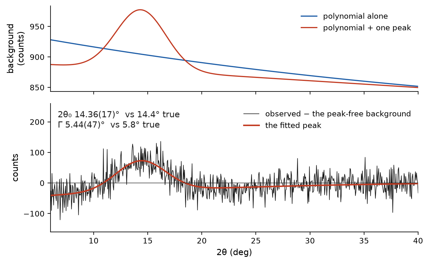
The pattern is synthetic, so its hump has a known position and width and the figure can say how close the three refined parameters came. The lower panel is the informative one: with the peak-free background subtracted, what is left is the feature, and the fitted peak lies along it.

Three parameters against three polynomial terms

A free position, height and width will lower any Rwp, which is exactly the kind of evidence this package does not accept. So the argument has to be two things at once: that the peak buys far more than the same number of polynomial terms buys, and that something outside the fit says what the feature is.

The pattern is tests/data/11BM_Si640c.xy, the same APS 11-BM scan of NIST SRM 640c silicon that tests/test_acceptance_si640c.py refines: run 4918, λ seeded at the header’s 0.412359 Å, 47 999 channels over 1.997–49.996° 2θ with the file’s own propagated esds. The specimen sits in a Kapton capillary, and Kapton scatters, so there is a broad envelope maximum near 5° 2θ that no Bragg peak of silicon accounts for. The protocol is that acceptance test’s full-range fit, with the cell held at the NIST certificate, FCJ axial divergence tied, lor_size and lor_strain on the phase, dispersion off, and λ and Biso freed last. The background is swapped from its P-spline to a low-order Chebyshev, and in the peak arms one HumpComponent is freed after the first stage and polished jointly with the polynomial at the end.

background	free background terms	Rwp	GoF	Biso(Si) / Ų	HIGH_CORRELATION
Chebyshev, 3 terms	3	0.119977	1.9695	0.414(75)	0
Chebyshev-3 + one hump	3 + 3	0.082503	1.3544	0.421(12)	0
Chebyshev, 6 terms	6	0.088597	1.4545	0.422(29)	0
Chebyshev-6 + one hump	6 + 3	0.077152	1.2666	0.4235(85)	0

Three peak parameters beat three polynomial ones. The first two rows differ by three numbers, and so do the first and third: three peak parameters against three extra polynomial coefficients, the same cost to the same fit. The peak takes Rwp from 0.119977 to 0.082503, a fall of 0.037 or 31 % relative; three more Chebyshev terms take it to 0.088597, 26 %. That is the whole comparison, and it is a fair one only because the parameter counts match.

The peak releases the Bragg intensity instead of competing with it. Biso(Si) barely moves, 0.414 to 0.421 Ų, well inside one esd. Its esd falls by a factor of six, 0.075 to 0.012 Ų. So do the esds of everything the background was trading against: λ 5.9×, the scale 6.0×, the zero shift 5.9×. A background the model cannot describe blurs this fit more than it biases it, and the three numbers that describe the hump give back the precision.

The fitted peak comes back at position 4.18(11)°, height 115.3(38) counts, FWHM 5.57(27)°. The instrumental Gaussian FWHM at that angle, from this fit’s own refined u, v, w, is 0.00346°, so the peak is 1 608× the resolution. That is what a diffuse feature looks like, and it is 400× clear of the HUMP_TOO_NARROW guard in the next section. Neither peak arm returns a single HIGH_CORRELATION finding.

The hump is the container, on three independent legs

Rwp cannot tell a container halo from a missed reflection. Three things outside this fit can.

The blank. 11-BM’s published standards listing carries run 4736 from the same February 2010 beamtime, header Chemical formula = empty Kapton capillary (Kapton), which is the container with no sample in it. It is tests/data/11BM_Kapton.xy. Fitted independently of this package (numpy Chebyshev, scipy least-squares, the file’s own σ) over the same 1.997–49.996° range, a 3-term Chebyshev plus one Gaussian reaches χ²ᵣ = 1.125 on 48 000 channels at position 4.2417(111)°, FWHM 6.153(23)°. Chebyshev-3 alone reaches only 5.33, and it takes fourteen polynomial terms, eleven more than the Gaussian’s three, for a peak-free polynomial to match those six parameters. Two codes, two scans, one feature, agreeing on position to 0.06° and on width to 0.6°.

The air-scatter control. The same listing carries a “No sample, Air Scatter Only” scan. Binned over 2–50° it decays strictly monotonically, bin after bin, with nothing localised anywhere, so the hump is in neither the beam nor the air path. It is the container. (That scan was taken at a different wavelength, so the claim has to be “no feature anywhere” rather than “no feature at 5°”: at 0.458735 Å the same d-spacing would sit at 5.56°, and the stronger form is free of that.)

The physics. The envelope maximum of the blank sits at 4.98° 2θ, which at that scan’s 0.412225 Å is d = 4.74 Å, Q = 1.33 Å⁻¹: the polyimide amorphous halo.

Together those make the peak a description of a known scatterer rather than a three-parameter Rwp reduction, and that is what makes this feature quotable.

Where the fitted centre is not the halo position

Read the table honestly and one number does not fit. The halo is at 4.98–5.05° by envelope, and the refined peak comes back at 4.18(11)°. The two are answering different questions.

A symmetric Gaussian spanning 2–50° has to absorb whatever the 3-term polynomial cannot, and what the polynomial cannot do at this end of the range is the residual direct-beam rise below 3°. So the fitted centre is pulled low. It is the best single Gaussian for the halo plus that rise, and not a measurement of the halo. Give the polynomial three more terms and the rise becomes the polynomial’s job: the Chebyshev-6 arm’s peak relaxes to 5.245(41)°, onto the envelope, and narrows from 5.57(27)° to 1.94(11)°.

Quote the envelope, and the blank, for where the halo is. Quote the fit for the model that describes it. Do not read the refined position as a physical d-spacing.

The same arithmetic is where one standing rule comes from. Between the Chebyshev-3 and Chebyshev-6 arms the peak moves 1.07° and changes width by a factor of nearly three while Rwp moves by 0.005. The peak and the polynomial are describing overlapping freedom, and the more flexible the polynomial, the less the peak’s own parameters mean. Declare a peak instead of extra polynomial terms, and if a peak’s parameters are what you intend to quote, keep the background as low-order as the fit tolerates.

What a hump is not

A free position, height and width is a peak with no cell and no structure factor behind it, and enough of those will improve any Rwp, which is exactly the kind of evidence this package does not accept. What makes the term a background term is that its width comes from disorder rather than from the goniometer, and disorder is many times the resolution. The case above is 5.57° wide where this synchrotron’s Gaussian FWHM at the same angle is 0.00346°, a factor of 1 608. A laboratory or neutron instrument will show a smaller ratio, the same Kapton halo against 0.3° lines being a factor of 20, and the guard is set for that weaker case.

So a peak that refines to less than HUMP_MIN_WIDTH_MULT (4.0) times the instrumental FWHM at its own position comes back with a HUMP_TOO_NARROW diagnostic. The reading is “these humps are not quotable”, the same reading STEPHENS_STRAIN_NOT_POSITIVE has and for the same reason: the condition depends on refinable parameters and on the peak’s own position, so it cannot be a bound the solver is handed. Use a hump for diffuse or amorphous scattering, or a cryostat, can or holder contribution. If there is a real unindexed line at that angle, the honest answers are a second phase or the unmatched-peak report in the FitReport’s Layer 0.

from rietx import Instrument
from rietx.schemas.common import Parameter
from rietx.schemas.instrument import HUMP_FWHM_MIN, HumpComponent

instrument = Instrument.debye_scherrer(wavelength=0.412359)
# seeded at the envelope, not at the value the fit above converged to: a seed
# is a starting guess, and the halo is where the blank says it is
instrument.extra_components = [HumpComponent(
    label="Kapton halo",
    position=Parameter(value=5.0, unit="deg"),
    height=Parameter(value=50.0, min=0.0, unit="counts", transform="softplus"),
    fwhm=Parameter(value=2.0, min=HUMP_FWHM_MIN, unit="deg",
                   transform="softplus"))]
assert len(instrument.extra_components) == 1

The paths are instrument.extra_components.*, one position, height and fwhm per declared peak, indexed by its place in the list, so relabelling a peak never moves its refined values. Note the underscore. instrument.background.*, which every preset’s first stage frees, does not reach them, because fnmatch’s * crosses dots and a nested spelling would have been freed at stage 1, with a free position over a pattern whose peaks had not been placed yet.

Calibrating an instrument once and reusing it

The instrument ⊕ sample split works only when the instrument half comes from somewhere other than the sample you are measuring. The workflow is three steps, and the middle one is a file.

1. Calibrate on a line-profile standard with its certified cell held fixed. That is what decorrelates the zero shift from the specimen displacement from the cell. The lab_calibrate plan frees the scale and background, then the zero shift and displacement, then the five width terms, then the emission-line weights and the axial ratios, then the displacement parameters. It never frees phases.*.cell.*, which is the whole point of using a standard.

2. Freeze with save_instrument_profile, which writes the calibrated state as JSON and strips what belongs to the measurement rather than the goniometer: the background, the specimen displacement and transparency, the surface roughness, and the specimen absorption.

3. Refine the sample from load_instrument_profile, which returns an Instrument with every stored parameter fixed. The lab_sample_refine plan frees the scale and background, the specimen displacement, the cell, the four sample broadening terms with the anisotropic strain block, the displacement parameters, and the surface roughness. It never frees the zero shift or the instrument widths, which arrived as data.

Step 2 strips those fields for a specific reason. Roughness is a property of how one specimen was packed and pressed, and µt of how thick one mount is, so carrying either into the next sample would pre-bias that sample’s displacement parameters, which is the bias these corrections exist to remove.

Files and projects has the calls and the file. What matters here is what a loaded profile means: the calibration is data, so it arrives fixed, and freeing it again on a sample undoes the decorrelation the standard bought.