A first refinement

A fit takes three objects and returns one. You supply a PatternData from read_pattern, a Structure from a CIF, and an Instrument that describes the diffractometer. The package returns a RefinementResult.

Throughout this manual, the examples/ scripts, and the API calls the history prints back at you, rietx is imported as rx.

The minimal call

import rietx as rx

data = rx.read_pattern("my_sample.xye")
structure = rx.Structure.from_cif("my_phase.cif")
instrument = rx.Instrument.debye_scherrer(wavelength=0.4139090)

result = rx.refine(data, structure, instrument)
print(result.status, result.statistics.rwp)

The print line writes two values:

converged 0.0932

RefinementResult.status is a plain string, one of converged, max_iter and diverged. The second of those means the solver ran out of iterations. It does not mean the fit failed.

Statistics.rwp is a fraction, not a percentage. 0.0932 is the Rwp of 9.3 % you would quote in a paper. Every R-factor in the package is stored this way. Reading the numbers says what each statistic measures.

One more line draws the fit:

result.plot(path="my_sample.png", two_theta_range=(2.0, 12.0),
            wavelength=0.4139090)

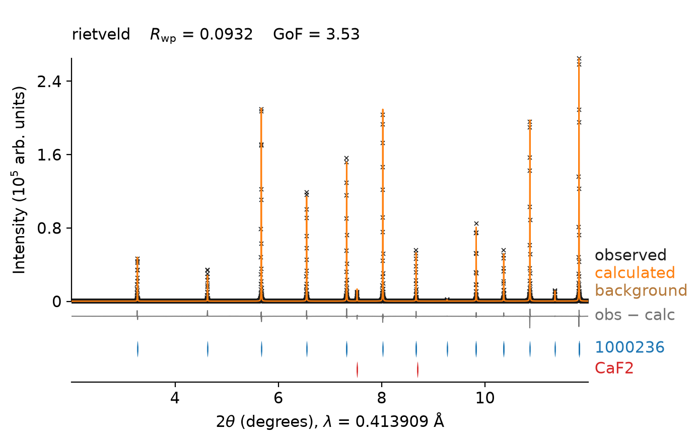
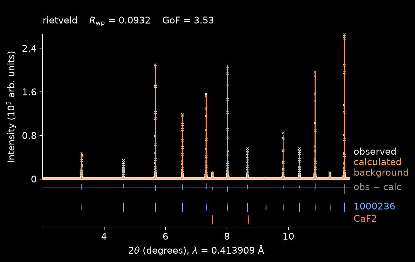
Reading down: observed points, the calculated line, the obs − calc difference on the same axis at the same scale, then one row of reflection ticks per phase. The residual sits directly under the peaks that caused it, and nothing comes between them. Every series is named in the right-hand margin rather than in a legend the eye has to look up; the fit statistics sit in the corner, because a figure’s title is its caption. two_theta_range is a window, not a crop — the intensity scale and the rows below it are built from what the window contains, so a zoom into a weak region is a figure of its own data.

weighted=True draws Δ/σ instead, in its own panel with a ±3σ band: a raw difference shares the intensity axis, so the eye reads a small deviation on a strong peak as a large error, while Δ/σ has expectation 1 under a correct model and the band is an absolute scale rather than a relative one. It is not the default because it costs the one thing the classic layout gives away free — the residual and the peak that caused it in a single glance.

wavelength= puts λ on the 2θ axis, which is meaningless without it; the result does not carry the emission line, so it has to be passed. It is also what x_axis="q" and x_axis="d" are derived through, and those two carry no λ of their own — that is the point of them. y_scale= takes "sqrt" (equal display distance for equal counting σ), "log" or "asinh"; any of them moves the difference into its own panel, since an offset raw difference is negative by construction and a nonlinear intensity axis cannot draw it. style="dark" is for a figure going onto a dark page, and figsize=/font_size= are the exposure surface: build the figure at the width it will be read at rather than scaling it in the document afterwards.

refine or a Refinement session

refine runs one fit and discards the session. It is the right call when one fit is all you need, and it keeps no history unless you ask for one (history=True).

The object form keeps the session:

ref = rx.Refinement(structure, instrument)
result = ref.fit(data, plan="mccusker_default")
result = ref.fit(data, plan="mccusker_structural")   # continues from the first

Refinement holds the models between calls, so the second fit starts where the first stopped rather than from the CIF. Three things come with that:

• Refinement.fitted_structure and Refinement.fitted_instrument return the models as the last fit left them.

• Refinement.history records every stage as a restorable node, and it is on by default here. Refinement.edit puts a change to the model on the same record, so adding a phase is a recorded move rather than a fresh start. The refinement history is what a node holds and how to go back to one.

• Refinement.report builds the FitReport with the compiled model attached, which build_report on a bare result cannot do.

Reach for the object form as soon as a fit needs a second attempt, which in practice is most of the time.

Le Bail before Rietveld

One decision matters more than any plan: get the peaks into the right places before you ask a structure to explain their intensities.

A Le Bail fit (mode="lebail") refines the cell, the zero shift and the profile with the intensities extracted per reflection instead of computed from the structure. It therefore converges from a much worse start, and it tells you whether the cell and the profile are right independently of whether the structure is. Only then does a Rietveld fit (mode="rietveld", the default) face a fair question. This is the IUCr guidelines’ own advice for a partial or uncertain model [MVDC+99].

It pays a second time. A Le Bail report flags observed peaks the model does not account for, so an impurity phase shows up as unmatched peaks at positions you can identify — before it can distort a structural refinement by being absorbed into a background or a width.

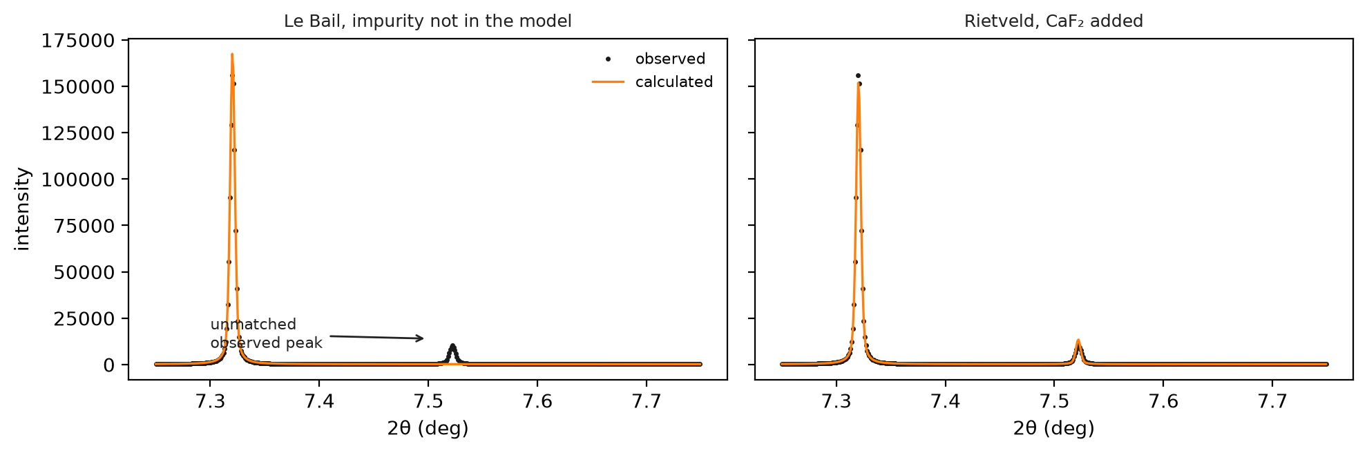
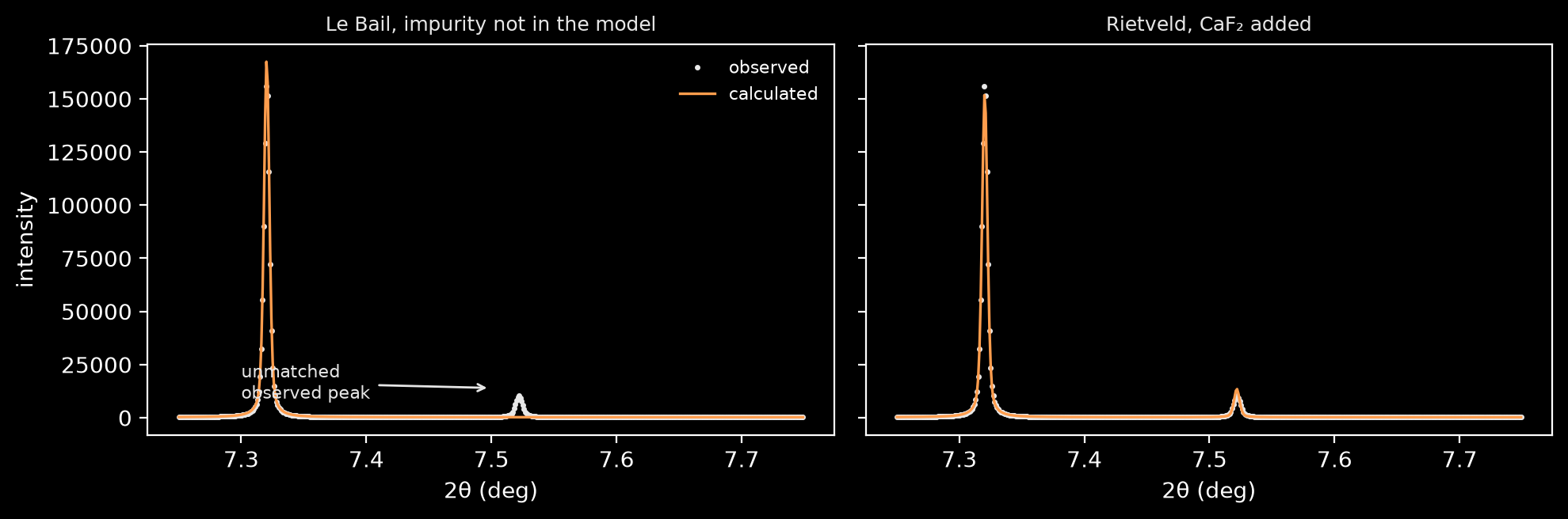
That is the mechanism in one picture, from the worked example below. The Le Bail fit knows nothing about CaF₂, so the line at 7.52° is observed intensity the model cannot place, and the report says so. Adding the phase accounts for it.

Worked example: NAC on 11-BM

This is examples/nac_11bm.py, which the test suite runs on every push. It refines Na₂Ca₃Al₂F₁₄ against APS 11-BM synchrotron data: Le Bail first, then the CaF₂ impurity its report exposes, then Rietveld.

Listing 1 examples/nac_11bm.py

"""v0.1 acceptance: Le Bail + Rietveld of NAC (Na2Ca3Al2F14) at APS 11-BM.

Data: GSAS-II tutorials, 11BM_NAC.fxye (λ = 0.4139090 Å from 11bm_gsas.prm).
Structure: COD 1000236 (Courbion & Ferey, 1988), cubic I2₁3, a = 10.257 Å.
"""

from pathlib import Path

import rietx as rx

DATA = Path(__file__).resolve().parent.parent / "tests" / "data"
WAVELENGTH = 0.4139090  # from 11bm_gsas.prm (INS 1 ICONS)


def run() -> tuple[rx.PatternData, rx.Refinement, rx.RefinementResult, rx.RefinementResult]:
    """The refinement itself, so that anything else needing these results —
    `docs/manual/make_figures.py` draws the manual's figures from them — reuses
    this script rather than keeping a second copy of the walkthrough."""
    data = rx.read_pattern(DATA / "11BM_NAC.fxye")
    print(f"pattern: {len(data.two_theta)} points, "
          f"{data.two_theta[0]:.2f}-{data.two_theta[-1]:.2f} deg, "
          f"sigma from file: {data.sigma is not None}")

    structure = rx.Structure.from_cif(str(DATA / "cod_1000236.cif"))
    phase = structure.phases[0]
    print(f"phase: {phase.name}, {phase.space_group}, a={phase.cell.a.value} A, "
          f"{len(phase.atoms)} asymmetric atoms")

    instrument = rx.Instrument.debye_scherrer(wavelength=WAVELENGTH)
    # starting profile guesses in the right decade for 11-BM resolution
    instrument.profile.w.value = 2e-5
    instrument.profile.x.value = 2e-3
    from rietx.schemas.instrument import BackgroundChebyshev
    instrument.background = BackgroundChebyshev.with_terms(6)

    limits = (2.0, 24.0)

    # --- Le Bail first: cell + profile without the structure
    # One Refinement carries the whole session; every stage auto-commits a
    # node, so `ref.history` ends up holding both refinements and the model
    # edit between them.  Pass history="nac.jsonl" to persist it.
    ref = rx.Refinement(structure, instrument)
    lebail = ref.fit(data, mode="lebail", two_theta_limits=limits)
    ref.history.tag(lebail.node_id, "lebail")
    a_lb = ref.fitted_structure.phases[0].cell.a.value
    print(f"\nLe Bail:  status={lebail.status}  Rwp={lebail.statistics.rwp:.4f}  "
          f"GoF={lebail.statistics.gof:.2f}  a={a_lb:.6f} A")

    # --- Rietveld seeded with the Le Bail cell/profile
    # The Le Bail FitReport flags unmatched observed peaks at 7.5, 12.3, 14.4
    # and 21.3 deg — exactly the fluorite 111/220/311/422 positions at this
    # wavelength: the classic CaF2 impurity in NAC synthesis.  Add it.
    structure2 = ref.fitted_structure.model_copy(deep=True)
    structure2.phases[0].scale.value = 1e-6
    structure2.phases.append(rx.Phase(
        name="CaF2",
        space_group="F m -3 m",
        cell=rx.Cell.cubic(5.4631),
        atoms=[
            rx.Atom(label="Ca", species="Ca2+", x=rx.Parameter(value=0.0),
                    y=rx.Parameter(value=0.0), z=rx.Parameter(value=0.0),
                    biso=rx.Parameter(value=0.6, min=0.0, max=25.0)),
            rx.Atom(label="F", species="F1-", x=rx.Parameter(value=0.25),
                    y=rx.Parameter(value=0.25), z=rx.Parameter(value=0.25),
                    biso=rx.Parameter(value=0.9, min=0.0, max=25.0)),
        ],
        scale=rx.Parameter(value=1e-7, min=0.0, transform="softplus"),
    ))
    # the impurity is a refinement move like any other — record it in the DAG
    ref.edit(structure=structure2, label="add CaF2 impurity phase")

    plan = rx.RefinementPlan.mccusker_default()
    plan.stages.append(rx.Stage("biso", ["phases.*.atoms.*.biso"]))
    result = ref.fit(data, plan=plan, two_theta_limits=limits)
    a = ref.fitted_structure.phases[0].cell.a.value
    a_err = result.parameter("phases.0.cell.a").stderr
    print(f"Rietveld: status={result.status}  Rwp={result.statistics.rwp:.4f}  "
          f"GoF={result.statistics.gof:.2f}")
    print(f"          a = {a:.6f} +/- {a_err if a_err else float('nan'):.6f} A "
          f"(COD reference 10.257(1); high-accuracy powder ~10.2497-10.2506)")
    for d in result.diagnostics:
        print(f"          [{d.level}] {d.code}: {d.message}")

    return data, ref, lebail, result


def main() -> None:
    _, ref, _, result = run()

    report = rx.build_report(result)
    print("\nFitReport:", report.summary)
    for r in report.regions[:5]:
        print(f"  region {r.two_theta_lo:6.2f}-{r.two_theta_hi:6.2f} deg  "
              f"localRwp={r.local_rwp:.3f}  chi2share={r.chi2_share:.1%}  "
              f"max|d/sig|={r.max_abs_delta_over_sigma:.1f}")

    print("\nRefinement history (every stage is a restorable checkpoint):")
    print(ref.history.summary())
    print(f"\nbest node by Rwp: {ref.history.best('rwp').id}")
    print("to revisit the Le Bail state:  ref.checkout('lebail')")

    try:
        result.plot(path=str(Path(__file__).parent / "nac_fit.png"),
                    two_theta_range=(2.0, 12.0), wavelength=WAVELENGTH)
        print("\nplot written to examples/nac_fit.png")
    except ImportError:
        pass


if __name__ == "__main__":
    main()

Six things in it recur in every fit after this one:

• One Refinement is the session. Refinement.fit can be called again, and the models carry over.

• Every stage commits a node. Refinement.history holds both refinements and the model edit between them, and RefinementTree.tag names a node to come back to. The refinement history is the whole record.

• A plan is editable. plan.stages.append(rx.Stage("biso", [...])) adds a displacement stage after the preset’s, and Stage takes fnmatch globs over the parameter dot-paths (phases.*.atoms.*.biso). The parameter table is the path grammar and how to see which paths a glob actually reaches.

• RefinementResult.parameter looks one parameter up by path, with its esd: result.parameter("phases.0.cell.a").stderr.

• RefinementResult.diagnostics is the channel for “your answer is wrong although Rwp is fine”. Read it every time. Reading the numbers says what a diagnostic carries, beside the statistics it outranks.

• build_report turns the result into a FitReport: where the misfit is, what would fix it, and whether the package is confident enough to say so.

The RefinementResult object

RefinementResult.status says whether the solver converged. RefinementResult.statistics carries the agreement indices, of which Statistics.rwp and Statistics.gof are the two usually quoted, and Statistics.n_points, Statistics.n_free_parameters and Statistics.esd_inflation are what make them interpretable.

The curves are on the result as RefinementResult.y_obs, RefinementResult.y_calc and RefinementResult.y_background, over RefinementResult.two_theta. RefinementResult.plot writes an observed/calculated/difference figure with matplotlib (the viz extra). Reading the numbers goes through the rest of the object field by field — the structure R-factors, the bonding geometry, and the two counts that say whether the pattern supported the model.

Rwp is not the answer. It is a fit statistic, and this package can show you a fit whose Rwp improved while its displacement parameters and phase fractions moved away from the truth. What the package hands you instead is the report.

Your own data

The script above builds its structure and instrument in code, which is the shortest way to show a whole fit. Patterns, structures and instruments is the reference for doing that with your own experiment: what each field of PatternData, Structure and Instrument means, which of the three instrument presets matches your diffractometer, and how to calibrate one on a standard and reuse it. Files and projects is the same ground from the file side, for data you already have on disk.